Download
1 / 38
380 likes | 552 Views
6 th “Georgian-German School and Workshop in Basic Science” GGSWBS’14 July 6-12 2014, Tbilisi, Georgia. On Numerical Modelling of Regional Atmospheric Processes over the Caucasus Teimuraz Davitashvili , Demuri Demetrashvili

E N D
6th “Georgian-German School and Workshop in Basic Science” GGSWBS’14July 6-12 2014, Tbilisi, Georgia On Numerical Modelling of Regional Atmospheric Processes over the Caucasus TeimurazDavitashvili, DemuriDemetrashvili I.Vekua Institute of Applied Mathematics of IvaneJanakhishvili Tbilisi State University; Institute of Geophysics of IvaneJanakhishvili Tbilisi State University tedavitashvili@gmail.comdemetr_48@yahoo.com Acknowledgment The work was supported by the 7th Framework Programme "SEE-GRID e-Infrastructure for regional e-Science", and the Georgian National Science Foundation Grant #GNSF/ST09/5-211.
Part 1. Modeling Study of Meso-scale Air flow Over the Mountainous Relief with Variable-in-Time Large-scale Background Flow. Part 2.Implantation of WRF-ARW Model for Caucasus Region Within European Commission’s 7th Framework Programme.
Georgia, as the whole Caucasian region is characterized by very complex topography. Such complex character of the relief and the vicinity of the Black and Caspian seas considerably deforms large-scale (synoptic) processes and causes formation of local and regional peculiarities of atmospheric processes and strong spatial inhomogeneity of meteorological fields Relief of Georgia It is well known that large-scale (synoptic) atmospheric processes are nonstationary. It is obvious, the question arises as to how the meso-scale flow over the complex terrain responds to the variability of large-scale processes. This question is very important for physical – geographical conditions of Georgia. Among synoptic processes developed above the territory of Georgia the western and eastern synoptic processes are very important. At western processes intrusion of air masses from the west to the east takes place, but at eastern processes air masses are moving from the east to the west. Observations show that in some cases the western air flow can be transformed to the eastern flow and on the contrary during short time period - 8-12 hours. To answer the question how the mesoscale flow over mountains responds to the sharp transformation of synoptic processes we used a 3-D hydrostatic nonstationary model of meso-scale processes for “ dry atmosphere”.
Description of the Model We consider moving air mass in the troposphere above the orographically inhomogeneous earth’s surface which from above at height of the tropopause is Limited by the free surface changeability of which is defined during integration of the model equations. As a result of influence of the relief the spatial - temporary distribution of meteorological fields essentially changes. Troposphere Schematic vertical section of the modeling area
After transition to the terrain-following system : Model equation system has the following form: , , , , v = V + v’, w = ,
Bboundary and initial conditions On the lower boundary ) ( At height of the troposphere On the lateral boundaries At the initial time t = 0
Numerical experiments Before carrying out numerical experiments of air flow over the real relief, we have considered the air flow over the isolated obstacle of a circular form. (a) the obstacle was given by formula Key parameters a0 = 1 km, r0 = 75 km, H0 = 12 km, l = 10-4 s-1 s = 0.003 K/m On a vertical 21 levels were taken by regular steps on each level there were 46 x 66 grid points.
Changeability in time of the background uniform flow During decreasing of air motion of synoptic scales (10 ÷ 16 h) from 12 m/s up to zero meso-scale disturbed flow is considerably transformed.In particular, the meso-scale wave current loses stability and amplitudes of wave current above the obstacle considerably grow in all troposphere. The wave current is gradually transformed into vortical current over the obstacle and at the moment of disappearance of the background current, the meso-scale motion can exist. t = 10 h t =10 h t = 14 h t = 15 h t = 24 h t = 16 h t = 17 h
t = 10 h Verticalvelocity disturbed temperature The fields of vertical velocitycomponent and disturbed temperature in the vertical section. From these figures it is well visible, that the upstream and downstream currents alternate with height, zones of cooling and warming accordingly alternate.
Air flow over the isolated obstacle on horizon z = 500 m t = 10 h t = 14 h t = 15 h t = 16 h t = 17 h t = 26 h At approach to the obstacle the air current is split on two branches.During decreasing of the background current speedthe deviations of the dersturbed meso-scale flow from the basic understurbed direction are increased. At the moment of time, when the background current completely disappears, the meso-scale movement above the obstacle continues to be existed.
Modeling of air flow above the real relief of Caucasus when the western background flow with speed U=12 m/s was transformed into the eastern flow with -12 m/s t =10 h t =15 h t =16 h t =17 h t = 28 h t =19 h During reduction of speed of the background flow from 12 m/s to 0, orographycaly disturbed flow undergoes significant changes. Above the Kolkheti lowland and the east part of the Black Sea the wind turns to the left counter-clockwise and tendency of generation of vortical formation is clearly observed. There is also interesting phenomenon, when the disturbed flow exists in spite of the fact that the background current is absent.
Modeling of air flow above the real relief of Caucasus when the western background flow with speed U=12 m/s was transformed into the eastern flow with -12 m/s t =10 h t =15 h t =17 h t =19 h It is visible that as in the case of model relief, the ordered wave current is gradually • transformed to the disorder movement with the tendency of vortex formations during decreasing of the large-scale flow. The disorder disturbed motion above the relief becomes ordered under the influence of occurrence of the background large-scale flow.
C O N C L U S I O N Performed numerical experiments in case of both model and real relief of Georgia have promoted some regularities of orographic effects caused by the nonstationarity of the large-scale background flow. During reduction of background speed up to zero the wave current above mountains loses stability, therefore the amplitudes grow and the wave current is gradually transformed to vortical movement. In case of disappearance of the background current the meso-scale circulation above the mountain relief does not disappear and exists during the certain time. The disorder disturbed motion above the mountain relief accepts the ordered character under the influence of occurrence of the background large-scale flow.
Part 2.Implantation of WRF-ARW Model for Caucasus Region Within European Commission’s 7th Framework Programme. OUTLINE • Introduction • Some features of SEE-GRID-SCI infrastructure and about European Commission's Seventh Framework Programme • Some features of WRF-ARW model • On implantation of WRF-ARW model in the SEE-GRID-SCI infrastructure • On implantation of WRF-ARW model for Caucasus region • Some results of calculations in the SEE-GRID-SCI infrastructure • Conclusions
FP7 Research InfrastructuresSEE-GRID-SCISEE-GRID eInfrastructure for regional eScience • Fig.1. The domain considered for SEE-GRID eInfrastructure development for regional eScience. • The work was carried out within the SEE-GRID project. • The SEE-GRID-SCI project was funded by the European Commission's Seventh Framework Programme for development Capacities-Research Infrastructures. • SEE-GRID-SCI project kicked-off in May 2008 and was completed by April 2010. • The projectwas coordinated by Greece NET (GRNET) with 14 contractors participating in the project:Albania, Armenia, Bosnia-Herzegovina, Bulgaria, Croatia, FYR of Macedonia, Georgia, Hungary, Moldova, Montenegro, Romania, Serbia, Turkey, and CERN(has a consulting role). • The total budget of the project was 3.214.689 €.
The main aims of the SEE-GRID-SCI project • Stimulation widening e-Infrastructure,inclusion new user groups from SEE countries; • Fostering collaboration and providing advanced capabilities to more researchers, with an emphasis on strategic groups in seismology, meteorology and environmental protection; • Further strengthen and widen the regional and national-level Human Network; • Provision of the network link to Moldova, so as to cater for immediate connection to Romania and thus to the rest of the region and Europe. • Inclusion of the Caucasus region in the infrastructure, namely Armenia and Georgia. • Ensure that all participating countries in the region will be mature enough for inclusion in the next-generation Grid operations model;
Meteorological Strategic Groups and their Role in the Project: • RudjerBoskovic Institute from Zagreb. Role in the projectwascoordination and leading development of application; Porting model to grid, fine-tunning; • Department of Geophysics, Faculty of Science, University of Zagreb. Model development and testing; • Faculty of Geophysics of Zagreb University. Inspecting post-processing possibilities (visualization); • Faculty of Electrical Engineering, University of Banja Luka, Bosnia. Porting model to grid and fine-tuning; • Republic Hydrometeorological Institute of Sarajevo. Developing and testing • Federal Hydrometeorology Institute, Sarajevo. Developing and testing, know-how; • and a new comer-Georgian Research and Educational Networking Association –GRENA.Developing and testing, know-how.
SEE-GRID-SCISEE-GRID eInfrastructure for regional eScienceGeorgian Research and Educational Networks Association (GRENA) team • RamazKvatadze (GRENA- Leader of the Georgian team). He is director of the GRENA • TemuriDavitashvili (VIAM;HMI-Leader of the meteorological group and chargeable for meteorological application ) • GeorgiKobiashvili(GRENA- administrator of the team; he was chargeable to create local cluster in GRENA) • NatoKutaladze(HMD-her role was developing and testing the meteorological application) • GeorgiMikuchadze(HMD- his role was to Porte the WRF-ARW into the SEE-GRID-SCIeInfrastructure and testing)
Meteorological Tasks-Applications in meteorology • In the frame of SEE-GRID project two meteorological applications were developed: • Regional scale multi-model, multi-analysis Ensemble Forecasting System – (REFS) • BOLAM, MM5, NMM, Eta models (multi-model system) • The main aim was developing a post-processing procedure, based on capabilities of the Grid infrastructure, collection and analyses the outputs from all models for forecasts over the area of central and eastern Mediterranean. Weather Research Forecast-Advanced Research Weather (WRF-ARW) Forecasting over the territory of Georgia: air temperature, quantitative precipitations, surface maximum wind speed, etc. Investigation peculiarities of interaction of airflow with complex orography of Caucasus using WRF-ARW model :
Creation of the Weather Research and Forecast (WRF) model • The WRF model has developed as a collaborative effort of the • Division of the National Oceanic and Atmospheric Administration’s (NOAA) • National Centers for Environmental Prediction (NCEP) and Forecast System Laboratory (FSL) of the USA • The Department of Defense’s Air Force of the USA. • Weather Agency (AFWA) and Naval Research Laboratory (NRL) • The Center for Analysis and Prediction of Storms (CAPS) at the University of Oklahoma • the Federal Aviation Administration (FAA), along with the participation of a number of university scientists. TheWRF model was first constracted in 2000 and today it has reached version 3. WRF modeling system was intended to provide a next-generation of mesoscale forecast model and data assimilation system, for understanding and prediction of mesoscale weather. The WRF model was designed to be configured for both research and operations. The WRF model is suitable for use in a broad spectrum of applications across scales from meters to thousands of kilometers.
WRFv3 ARW • As shown in the diagram, the WRF Modeling System consists of these major programs: • External data source-(terrestrial data and gridded data) • • The WRF Preprocessing System (WPS)-the role of WPS is to prepare input data • for real-data simulation and forecast. • • WRF-Var(variational data assimilation system) • • ARW model (solver) • • Post-processing & Visualization tools
ARW Solver-numerical scheme • Equations: Euler nonhydrostatic equations. The ARW equations are formulated using a terrain-following hydrostatic-pressure vertical coordinate denoted by Eta and defined as Eta= (ph−pht)/μ where μ = phs−pht. Fully compressible. • Prognostic Variables: Velocity components u and v in Cartesian coordinate, vertical velocity w, potential temperature T, geopotentialF, and surface pressure of dry air P., turbulent kinetic energy E, water vapor mixing ratio Mw, rain/snow mixing ratio Mr, and cloud water/ice mixing ratio Mc. • Horizontal Grid: Arakawa C-grid staggering. • Time Integration: Time-split integration using a 3rd order Runge-Kutta scheme with smaller time step for acoustic and gravity-wave modes. • Spatial Discretization: 2nd to 6th order advection options in horizontal and vertical.
The WRF physics schemes optionsare divides into several categories, each containing several options. The physics categories are:(1)microphysics; (2) cumulus parameterization; (3) planetary boundary layer (PBL); (4) land-surface model; (5) radiation. • Microphysics:Microphysics includes explicitly resolved water vapor, cloud, and precipitation processes. There are the following microphysics schemes in the WRF-AWR model: Kessler-3, Purdue Lin-6, WRF Single-Moment 3-class (WSM3), WSM5 WSM6, Eta-2, Thompson-7. For instance Six classes of hydrometeors are included: water vapor, cloud water, rain, cloud ice, snow, and graupel. • Cumulus parameterizations:These schemes are responsible for the sub-grid-scale effects of convective and/or shallow clouds.Kain-Fritsch,(Mass flux schem); Betts-Miller-Janjic (Adjustment) and Grell-Devenyi(Mass flux schem) • Surface layer physics: The surface layer schemes calculate friction velocities and exchange coefficients for calculation of surface heat and moisture fluxes by the land-surface models;similarity theory (MM5);similarityMonin-Obukhov, Zilintikevich,… schemes; • Land surface model: use atmospheric information from the surface layer scheme, radiative forcing from the radiation scheme, and precipitation forcing from the microphysics and convective schemes. 5-layer thermal diffusion;Noah LSM additionally predicts soil ice, and fractional snow cover effects, Rapid Update Cycle (RUC) Model LSM
The WRF physics schemes: (3) planetary boundary layer (PBL); (5) radiation. • Planetary boundary layer physics:is responsible for vertical sub-grid-scale fluxes due to eddy transports in the whole atmospheric column.CO2, O3, clouds.Medium Range Forecast Model (MRF) PBL; Yonsei University (YSU) PBL; Mellor-Yamada-Janjic (MYJ) PBL • Atmospheric Radiation: The radiation schemes provide atmospheric heating due to radiative flux divergence and surface downward long-wave and shortwave radiation for the ground heat budget.There are 5 schemes in the WRF model: Rapid Radiative Transfer Model (RRTM) Longwave- is taken from MM5; Eta Geophysical Fluid Dynamics Laboratory (GFDL) Longwave; Eta (GFDL) shortwave; MM5 (Dudhia) Shortwave; Goddard Shortwave. • Physics Interactions: it should be noted that there are many interactions between them via the model state variables (potential temperature, moisture, wind, etc.) and their tendencies, and via the surface fluxes.
ARW Solver-2 • Turbulent Mixing and Model Filters:Sub-grid scale turbulence. Divergence damping, external-mode filtering, vertically implicit acoustic step off-centering. Explicit filter option also available. • Initial Conditions:Three dimensional for real-data, and one-, two- and three-dimensional using idealized data. A number of test cases are provided. • Lateral Boundary Conditions: Periodic, open, symmetric, and specified options available. • Top Boundary Conditions:Gravity wave absorbing (diffusion or Rayleigh damping). w = 0 top boundary condition at constant pressure level. • Bottom Boundary Conditions:Physical or free-slip. • Earth’s Rotation:Full Coriolis terms included. • Mapping to Sphere:Three map projections are supported for real-data simulation: polar stereographic, Lambert-conformal, and Mercator. Curvature terms included. • Nesting:One-way, two-way, and moving nests. The basic essence of nesting modeling is to provide better resolution and reproduction of atmospheric processes for the region of our interest. With this purpose the calculated grid with fine resolution is nested in the coarser (parent) grid. The outputs of the model with coarse grid are used as lateral boundaries for the region of our interest.
The ARW supports horizontal nesting that allows resolution to be focused over a region of interest by introducing an additional grid (or grids) into the simulation. • In the current implementation, only horizontal nesting is available: there is no vertical nesting option. • The nested grids are rectangular and are aligned with the parent (coarser) grid within which they are nested. Additionally, the nested grids allow any integer spatial (_xcoarse/_xfine) and temporal refinements of the parent grid. • Fig. Various nest configurations for multiple grids: (a) left, Telescoping nests. (b) right, Nests at the same level with respect to a parent grid. Nesting 1 1 2 3 2 3 4
The 1-way and 2-way nesting options • Nested grid simulations can be produced using either 1-way nesting or 2-way nesting as outlined in the left Fig. The 1-way and 2-way nesting options refer to how a coarse grid and the fine grid interact. In both the 1-way and 2-way simulation modes, the fine grid boundary conditions (i.e., the lateral boundaries) are interpolated from the coarse grid forecast. • In a 1-way nest, this is the only information exchange between the grids (from coarse grid to fine grid). Hence, the name 1-way nesting. • In the 2-way nest integration, the fine grid solution replaces the coarse grid solution for coarse grid points that lie inside the fine grid. This information exchange between the grids is now in both directions (coarse-to-fine and fine-to-coarse). Hence, the name 2-way nesting. • The 1-way nest option may be run in one of two different methods.
Area of integration and nesting types • In numerical calculations outer domain covers the Caucasus region with 167x117 points in the north-south and east-west directions, respectively, with 15km mesh • Fig. shows area of integration and relief used into the model • Nested domain fixed in space over Georgia and contained 145x115 points with a 5-km mesh • The forecasts were integrated 24, 48 and 72 hours ahead using: • 1-way and 2-way nesting (with feedback) runs, also with moving nesting following the process of our interest
Moving nesting If our interest is to follow some atmospheric process (f.e., moving of cyclon center) moving nesting is used. In this case the fine grid follows this atmospheric process. For the moving fine grid with 1-way nesting the boundary conditions are specified by the parent grid at every coarse-grid time step (maximum amount of time steps is equal to 50). It is indicated identification number of the nested domain, time steps and moving directions along the X and Y axis's during the moving. The Fig. represents calculated values of the sea level pressure with cyclone center The Fig. represents moving of the nested grid domain automatically connected with moving of the cyclone center
Elaboration of WRF-ARW for Georgia’s Territory Porting NWP models on the GRID gave solution for following problems: Operational usage of the model; The possibility of storing large amount of data (grid storage elements); The possibility of producing more accurate forecast (better resolution, shorter time interval, etc...); • Limited area WRF-ARW model has been elaborated and configured for Caucasus region. • Implementation of the model required installation, configuration and compilation of operational environment in LINUX, which in turn required compilers (C, C++, Fortran) and scripting languages (Perl, Python), and other software libraries. Also building the program for multi-processor systems was necessary. • We have used the real time outputs of global model - GFS (Global Forecast System), as lateral boundary and initial conditions for regional domain.
WRF-ARW application for Georgia-Western Process Bellow are two case studies which are generally characterize model simulation behavior for western and eastern type synoptic processes • Fig.1 Initial map of sea level pressure and high clouds fields for 9 January 2009 (00 UTC) simulated for the main domain with 15 km resolution. • In the first case air masses sharply invasion was occurred from the Black Sea side, what was followed by strong winds in Tbilisi. The both 15-km outer domain and 5-km nested domain were used. Model equations were integrated at 00 UTC 9 Janury 2009. • As shown from the Fig.1, South-west of Caucasus is occupied by high pressure area and thus prevents eastward spread of low atmosphere pressure trough.
WRF-ARW application for Georgia-Western Process Fig.2 Surface pressure and high clouds prognostic map for 12 UTC 9 January 2009, simulated for the main domain with 15 km resolution • fig.2 indicate fast propagation of low pressure area from the Black Sea to eastward direction. • All upper air maps (925, 850, 700, 500 hpa) also have shown the same. • prognostic maps indicated that atmospheric front moving from the west to east direction passed Tbilisi in the afternoon of local time. • For that period biting changes of meteorological parameters were recorded in Tbilisi. Prognostic values of wind speed increased by height and reached 50-60 m/s at 850 hpa. • Despite quite strong frontal penetration as it was shown from prognostic maps of precipitation it’s unlike to foresee heavy rains in Georgia. The observed amount of rainfall actually was little.
WRF-ARW application for Georgia-Eastern Process In the second study the case of the eastern process observed in 05.11.2009 was examined. • Fig.3. Forecasted (3 Nov. 00 UTC) precipitation 12 h sum for nested domain with 2-way nesting method and 5 km resolution. • Fig.4. Forecasted (4 Nov. 00 UTC) precipitation 12 h sum for nested domain with 2-way nesting method and 5 km resolution. • On the figures 3 and 4 forecasted precipitation fields are presented, where the figure 3 demonstrate 72 h WRF-ARW forecast failure when global models predicted dray conditions, as well as the observed precipitation. • The next figure shows forecast of the above mentioned field integrated from 4 Nov. 00 UTC (48 h) which was in better agreement with observations. • Based on experience it can be said that the capture of eastern and southern processes are the most difficult issue for NWP models, when main difficulties raised during the prediction of spatial-temporal distribution of precipitation fields.
A COMPARISON OF CUMULUS PARAMETERIZATION SCHEMES IN THE WRF MODEL • WRF-ARW modeling system allows to use different convection parameterization and microphysical schemes. Therefore there is a question of sensitivity of the modeling system to different schemes in the conditions of the complex relief of the Caucasus. Such researches were carried out within this project. • The WRF-ARW version 3.1 model was running operationally on the SEEGRID during several months with four different model configuration combining 2 different convective and 2 microphysical schemes: • Betts-Miller-Janjic(BMJ) parameterization, with Lin microphysics scheme. • BMJ- convection scheme with WRF single-moment 6 class microphysics scheme. • Kain-Fritsch scheme (KF), combined with Lin microphysics scheme. • KF- combined with WRF single-moment 6 class microphysics scheme. • All simulations used the Yonsei University Planetary boundary layer schemes, 5-layer soil model for Surface layer and Dudhia’s Shortwave and RRTM Long wave radiation schemes. • The model performance was carried out with two way nesting option.
Min. temperature at the 2m level- computed by model and observed MMin. temperature at the 2m level- computed by model (with accounting of Var. Assimilation) and observed Min. temperature at the 2m level- computed by model and observed MMin. temperature at the 2m level- computed by model (with accounting of Var. Assimilation) and observed
Conclusion • In summary it can be said, that above mentioned model can be successfully used for local weather prediction for western type synoptic processes. • Though model results are more realistic in forecasting of prognostic variables characters, concerning to quantitative prediction of such variables as surface maximum wind speed, air temperature, etc. • statistical calibration should be done additionally. • for evolution and improvement of model skill for different time and spatial scale the verification and assimilation methods should be used for further tuning and fitting of model to local conditions.
Conclusion WRF-Nesting • Meso-scale phenomena (eastern invasion) was not simulated correctly in time • Precipitation was forecasted 12 hours earlier and overestimated • Capture of factual situation WRF ARW could only 24 hours ahead • For 3-day forecast nesting does not improve precipitation forecast: overestimation was increased • For 2-day forecast there was some improvement using nesting: more detailed precipitation distribution