Numerical Analysis of Processes

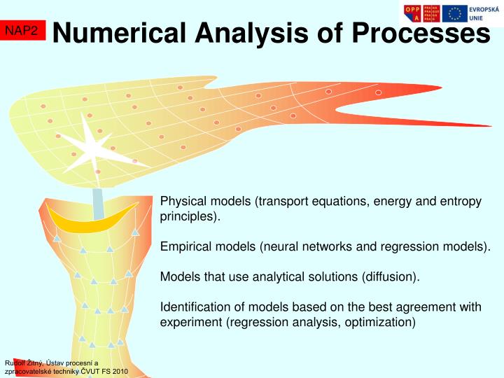
1. Numerical Analysis of Processes NAP2 Physical models (transport equations, energy and entropy principles). Empirical models (neural networks and regression models). Models that use analytical solutions (diffusion). Identification of models based on the best agreement with experiment (regression analysis, optimization) Rudolf Žitný, Ústav procesní a zpracovatelské techniky ČVUT FS 2010

2. Identification of the model parameters on the basis of experiment Mathematical model of an apparatus or system Experiment evaluationfor example diagnostics Optimisation of operational parameters Mathematical MODELs NAP2 Mathematical model = mathematical description (program) of system characteristics (distribution of temperature, velocity, pressure, concentration, performance, ...), as a function of time t, space and operating parameters (geometry system, material properties, flow, ...). Rudolf Žitný, Ústav procesní a zpracovatelské techniky ČVUT FS 2010

3. Mathematical MODELs NAP2 General classification of models • Black box - a model based solely on a comparison with experiment. Three basic types are • Neural networks (analogous neurons in the brain - the method of artificial intelligence) • Regression models (e.g. in the form of correlation functions of the power law type Nu = cRenPrm) • Identification of the transfer function of a system E(t) from the measured time history of input x(t) and output y (t) of the system. • White box - the model is based entirely on sound physical principles: • the balance of mass, momentum, energy (Fourier and Fick's equation, Navier Stokes equations) • on energy principles, the desired solution minimizes the total energy of the system (elasticity), • on simulations of random movements and interactions of fictitious particles (Monte Carlo, lattice Boltzmann ...).- • Grey box - models, which is located between the above extremes. Examples are compartment models of flow systems, respecting the physical principle of conservation of mass, but other principles (eg balance of momentum), they are replaced by empirical correlations or data. Rudolf Žitný, Ústav procesní a zpracovatelské techniky ČVUT FS 2010

4. Physical Principles NAP2 Continuum models (white boxes) Engineering models based on physical principles are often based on three balances (mass, momentum and energy). In differential form: Moss conservation Momentum conservation Energy conservation Cauchy equilibrium equations. Valid for structural as well as fluid flow analysis, compressible and incompressible. The total energy, the sum of internal, kinetic and potential energy power of inner forces heat flux Most of the equations, you know, can be derived from these conservation equations: Bernoulli, Euler, Navier Stokes, Fourier Kirchhoff.

5. Wi W(u) u We Physical Principles NAP2 Continuum models (white boxes) The principles of energy are preferred especially in the mechanics of solid phase.In the theory of elasticity it is the Lagrange principle of minimum of potential energy strains and stresses can be expressed in term of displacement u deformation energy of internal forces (the product of the stress and strain tensor work of external forces (volumetric, surface, concentrated) at equilibrium the energy (Wi+We) is minimum Requirement of zero variation of energy functionalW/u=0 is the basis of many finite elements design. This approach is represented in dynamics byHamilton principleof zero variation of functional with kinetic energy "Energy" principles are not so general: each of the variational principle can derive an equivalent Euler Lagrange differential equation, but the converse is not true. Especially with flow the variational principles can be applied only in some cases (eg creeping flow).

6. Physical principles NAP2 Models determine the type of engineers who are engaged in addressing these issues:FUNCTIONALISTS imagine that each system can have infinitely many forms, anda number, functional can be assigned to each of them. Then they plot these numbers and look for somespecial points (minima, maxima, inflection). A special mystical significance is assigned to these characteristic points, perhaps, the state of balance, loss of stability, etc. Functionalists work especially in mechanics of solids and are easily identified by the fact that they appretiate only the finite element method (through gritted teeth perhaps Boundary Elements).They use words as Cauchy Green tensor, Kirchhoff - Piola stresses, the seventh-invariant, etc.DIFFERENTIALs believe that the law of conservation of mass, momentum and energy expressed in terms of differential equations can describe the state of a system in the infinitesimal neighborhood of any point (and consequently the whole system too). When choosing numerical methods the differentials are not too picky, but generally choose the method of finite volumes. Often use words like material derivative.PARTICULARISTs do not believe in continuum mechanics. Everything can be derived from the mechanics of a particle. There are only discrete quantities, such as in digital computers. The complexity of reality is caused by a large number of simple processes running in parallel. Particularists can be identified by the fact that shuns all others and are discreet.FATALISTs do not believe that it is possible for a human beeing to understand the laws of God providence and therefore are limited to the empirical description of the observed phenomena. They love expert systems, artificial intelligence methods, engineering correlations and statistics.CHAOTs admit existence of some principles, but do not believe in their meaningful solvability. They hate the smooth curves, and prefer to be spoiled by random number generators. They love disasters, catastrophs and attractors. They are attractive especially for women fascinated by foreign words and colorful flowers of fractals.

7. Example of models Drying NAP2 As an examplewe will use different mathematical models of drying or moistening of the material, such as grain (starch, corn, rice, coffee ...) in the whole course. There will always be one of the basic results time of drying (or relationship between time, temperature and moisture of dried material). For this purpose simple regression models or neural networks are usually sufficient. The distribution of moisture within the grain must be known (calculated) as soon as the microbial activity or healt risc is to be determined. White or gray boxes models based on transport equations and heat diffusion can be used. When the grain has a simple geometry (ball), and when there is no significant effect of moisture on the diffusion coefficient, the solution can be expressed in the form of infinite series (analytical solution of Fick's equation and FK, only few terms in these series are sufficient). When the geometry is simple, but diffusion and heat transfer coefficients are strongly non-linear, the 1D numerical methods are preferred (finite difference method or the spectral method). The complicated shape of grains (rice, beans) are evaluated by 3D numerical finite element or control volume (commercial software ANSYS, COMSOL and FLUENT are usually used). At present, the concern is focused to changing internal structure of a material, such as cracking, which in turn significantly affect the moisture (free water easily penetrates micro grain). This means that in addition to transport equations the deformation field and the distribution of mechanical stress tensor (elastic problem) must be solved. These models are generally based on the finite element method. Rudolf Žitný, Ústav procesní a zpracovatelské techniky ČVUT FS 2010

8. Neuronové sítě NAP2 Artificial neural networks are the brutal techniques of artificial intelligence. Its popularity stems from the fact that more and more people know less and less about the real processes and their nature (maybe it could be called the law of exponential growth of ignorance). ANN (Artificial Neural Network) is designed specifically for those who knows nothing about the processes they want to model. They just have a lot of experimental data in which they are unable to navigate. And have a MATLAB (for example). Schiele

9. Valce controlling substrate flowrate 3 1 4 7 Sensors 5 2 6 NEURALNETWORK - BRAIN Neuron has several inlets - dendrits and one output - axon Neural Networks NAP2 Neuron=module that calculates one output value from several input. The behavior of a particular neural network is given by the values of the synaptic weights wi (coefficients amplification of signals between interconnected neurons) Hidden layer (here 4 neurons) Input layer (2 neurons) X1,X2 Outlet layer (1 neuron) Y Neuron’s responseyto N-inputsxi Wi=coefficients of synaptic weights evaluate by special algorithm „learning“ network The most frequently used activation functions f (tangens hyperbolic, sigmoidal function, sign function sgn). All implemented e.g. in MATLABu. Nejčastěji používané aktivační funkce f (tangens hyperbolický, sigmoidální funkce, znaménková funkce) Nejčastěji používané aktivační funkce f (tangens hyperbolický, sigmoidální funkce, znaménková funkce)

10. Neural networks NAP2 Modeling of wheat soaking using two artificial neural networks (MLP and RBF)Journal of Food Engineering, Volume 91, Issue 4, April 2009, Pages 602-607M. Kashaninejad, A.A. Dehghani, M. Kashiri In this article you will read how the experiments on cereal grains humidification were evaluated. Humidificated grains were in distilled water at temperatures of 25, 35, 45, 55 and 65 0C for about 15 hours (samples were weighed at 15 minute intervals), the total available 154 values of specific humidity of grain for various temperatures and times. From these values only the 99 data were used for training the network, which had two neurons in the input layer (time, temperature), 26 neurons in the hidden layer and a single output neuron (humidity). Remaining 55 data (moisture) was used to verify that the “trained" neural network gives reasonable results and what is about fault prediction. They used two types of network MLP (Multi Layer Perceptron) and RBF (Radial Base Functions) with different activation functions of neurons (sigmoidal, respectively. Gaussian basis function). This is prediction of neural network (ANN). MR-Moisture Ratio as a function of time and temperature. MLP is a classical neural network. Neuron activation function (hyperbolic tangent ... see previous film) with no adjustable parameters, optimize only the weighting coefficients wij connecting neuron with neuron j (and used the same method as described in further regression models). Radial basis function RBF neurons have their own adjustable parameters - coordinates of the neuron (determines the "distance" from the neuron of the previous layer neurons) and "width" basis functions. RBF is the Gaussian function RBF networks have only one hidden layer and weighting coefficients wij can be adjusted between the hidden and output layer. Parameters of the "radial" neurons (xc,  c) is selected "ad hoc" to the nature of the problem, while using the statistical strategy of "cluster analysis". It is more complicated than the MLP and the result (at least for drying) tends to be worse.

11. Regression models NAP2 Delvaux

12. Regression models NAP2 The regression model has the form of a relatively simple function of the independent variable x, and the parametersp1, p2,…,pM, which is to be determined so that the values of the function best match the experimental values y. . Frankly neural networks are almost the same.The search parametersp1, p2,…,pM are the coefficients of synaptic weights linking neurons. The difference is that the type of the model functions is more or less unified inthe ANN and the number of weights is greater than the number of parameters commonly used in regression functions. Regression function is chosen on the basis of experience or simplified ideas of modeled process (reasonable and logically explainable behavior at very small or large values of the independent variables is to be required). It is also desirable that the parameters p1, p2,…,pM have clearly defined physical meaning. However, it is true that if we do not know a physical nature of the process or if it is too complex (ie, the same situation as in neural networks) the polynomial regression function y= p1+p2x+…+pMxM-1or another „neutral“ function is used.

13. Regression models NAP2 Let us consider a regression model with the unknown vector p of M parameters The parameters pi should be calculated so that the model prediction best fits the N measured points (xi,yi). The most frequently used criterion of fit is chi-square (sum of squares of deviations) Number of data points N should be greater than the number of calculated parameters M (N=M means interpolation) The quantityiis standard deviation of measured quantity yi (measurement errror). Regression looks for minimum of the function 2in the parametric space p1, p2,…,pM (sometimes more robust criteria of fit, for example the sum of absolute values of deviations, are used). Quality of a selected model is evaluated by the so called correlation index, which should be close to unity for good models The worst val;ue r=0 corresponds to the case when it would be better to use a constant as a regression model )

14. Linear regression NAP2 Linear regression model is a linear combination of selected base functions, for example polynomialsgm(x)=xm-1or goniometric functionsgm(x)=sin(mx) Base functions are analogy of activation functions of neurons and the parameters pmcorrespond to synaptic weights. Model prediction can be expressed in a matrix form [[A]] is design matrix with N rows corresponding to N/points and M columns for M-base functions. N>M, the case of square matrix N=M is not regression but interpolation. As soon as the standard deviation is constant, the 2value is proportional to the sum of squares s2 ofdeviation between prediction[ypredikce] and measured data[y] This is scalar product of two vectors

15. Linear regression NAP2 Zero first derivatives of s2with respect of all model parameters exist at minimum which is the system of M linear algebraic equations for M unknown parameters Transposed matrix[[A]]Thaving dimension MxN multiplied by vector [y] Nx1 gives a vector of M-values Transposed matrix[[A]]Thas dimension MxN and when multiplied by [[A]]gives square matrix with the dimension MxM [[C]]MxM Matrix [[C]] enables estimate of reliability interval of calculated parameters p1,…,pM pkis standard deviation of calculated parameter pkfor k=1,2,…,M y jis standard deviation of measured data (it is assumed that all data are measured with the same accuracy) Inversion of matrix [[C]] (inverted matrix is called covariance matrix)

16. Linear regression– example noise filtration NAP2 Principle of Savitzky Golay filter of noised data is very simple:each point of input data xi,yiis associated with the window of Nwpoints left and Nwpoints right and these 2Nw+1 points is approximated by regression polynomial of degree k, where k<2Nw. Value of this regression polynomial in the point xisubstitutes original value yi. Number of data N=1024, width of windowNw=50, quadratic polynomial. The SG filtration is implemented in MATLAB as function SGOLAYFILT(X,K,F) where X vector of noised data, K degree of regression polynomial and F=2Nw+1 is width of window.

17. Regression modelsexample-soaking NAP2 Many empirical models are used for description of relationship between moisture content in grains and time, for example exponential Page’s model There are two model parameters p1=k, p2=n. Independent variable t is time Xeis equilibrium, XOinitial moisture of grain and even more frequently used Peleg’s model (see paper) Parameter p2 characterises equilibrium moisture The application of Peleg's equation to model water absorption during the soaking of red kidney beans (Phaseolus vulgaris L.)Journal of Food Engineering, Volume 32, Issue 4, June 1997, Pages 391-401Nissreen Abu-Ghannam, Brian McKenna Peleg’s model is usedfor beans, chickpeas, peas, nuts… Page and Peleg models are nonlinear and in practice are transformed to linear form by logarithm (Page)or (Peleg) as tvar This is new dependent variable y …and then linear regression can be applied for identification of p1 a p2

18. Regression models-soaking NAP2 Linearisation of non-linear models (for example linearisation of Page and Peleg models) means that the optimised parameters p1, p2 minimise some other criterion than the 2 and also other characteristics, like covariance matrix, correlation index do not correspond to the assumption of normal distribution of errors. However, this effect is usually small and can be neglected.

19. Analyticalsolution diffusion and heat NAP2 Vermeer

20. Analyticalsolutions NAP2 Analyticalsolution exist only at linear models Ordinary differential equations: Partial differential equations: there exist two ways any analytical functions that you know, for example sin, cos, exp, tgh, Bessel functions,… are defined in fact as a solution of ordinary differential equations (see handbooks, for example Kamke E: Differential Gleichungen, Abramowitz M., Stegun I.: Handbook of Mathematical functions). General approach consists in expression of solution in form of infinite power series and identification of coefficients by substitution the expansion into the solved differential equation Fourier method of separation of variables. Solution F(t,x,y,z) is searched in the form of product F=T(t)X(x)Y(y)Z(z). Substituting into partial differential equation results ordinary differential equations for T(t), X(x), Y(y) and Z(z). Application of integral transforms: Fourierovu, Laplaceovu, Hankelovu. Result is algebraic equation, which is to be solved and back-transformation must be used.

21. Analytical solutiondiffusion (1/5) NAP2 Distribution of moisture X (kg water/kg solid) is described by Fick’sequation Xeequilibrium, X0initial moisture m=0,1,2 for plate, cylinder, sphere. Fourier method of separation of variables Substituting to Fick’s PDE results in fact both terms must be constants independent on t, r. The constant is called eigenvalue. This term depends only on time t this terms depends only on r

22. Analytical solutiondiffusion (2/5) NAP2 Solution of Gi(t) is exponetial function, solution of Fi(r) is cos(r) for plate (m=0), Bessel function J0(r) for cylinder (m=1) and for sphere (m=2, this is our case of spherical grains) Phase equilibrium is assumed at the sphere surface (r*=1, X=Xe). Therefore X*(t,1)=0 and this condition must be satisfied by anyfunction Fi. This is the condition for eigenvalues Dimensionless con centration profile is therefore The coefficients ci must be selected so that the initial condition (distribution of concentration in time zero) will be satisfied. For constant initial concentration X=X0must hold X*=1 for arbitrary r*, thewrefore

23. Analytical solutiondiffusion (3/5) NAP2 The coefficients ciare evaluatred from orthogonality of functions Fi(r*). Functions are orthogonal if their scalar product is zero. Scalar product of functions is defined as integral Proof per partes integration. Thbis is zero because both functions F must satisfy boundary conditions

24. Analytical solutiondiffusion (4/5) NAP2 Let us apply orthogonality to previous equation (multiplied by r2Fj and integrated) Concetration profile or by integration across the volume of sphere total moisture content as a function of time

25. Analytical solutiondiffusion (5/5) NAP2 Diffusioncoefficient Defgeneraly depends upon temperature and moisture and also the equilibrioum moisture Xeis a function of temperature, for example Regression model is therefore strictly speaking nonlinear (with parameters p1=Dwa, p2=Ea a p3=b) and the analytical solution with substituted Def is only an approximation. This model used Katrin Burmester for coffee grains Heat and mass transfer during the coffee drying processJournal of Food Engineering, Volume 99, Issue 4, August 2010, Pages 430-436 Katrin Burmester, Rudolf Eggers Modeling and simulation of heat and mass transfer during drying of solids with hemispherical shell geometryComputers & Chemical Engineering, Volume 35, Issue 2, 9 February 2011, Pages 191-199I.I. Ruiz-López, H. Ruiz-Espinosa, M.L. Luna-Guevara, M.A. García-Alvarado

26. Optimalisation NAP2 • There are two basic optimisation techniques for calculation of parameters pi minimising 2of nonlinear models : • Without derivatives, when minimum can be identified only by repeated evaluation of s2 (or another criterion of fit between prediction and experiment) for arbitrary values of parameters pi. These methods are necessary at very complicated regression models, for example models based upon finite element methods. • Derivative methods, making use values of all first (and sometimes second) derivatives of regression model with respect to all parameters p1,p2,…,pM.

27. Optimisation methods with derivatives NAP2 Gauss method of least sum of squares of deviations Weight coefficients (representing for example variable accuracy of measurin method) model data Zero derivatives with respect all parameters j=1,2,…,M Linearisation of regression function by Taylor expansion p is increment of parameters in one iteration

28. Optimisation methods with derivatives NAP2 Solution of systém of linear equations in each iteration The most frequently used modification of Gauss method is the Marquardt Levenberg method : diagonal of matrix [[C]] is increased by adding a constant  in the case that the iteration are not converging. For very high  the matrix [[C]] is almost diagonal and the Gauss method reduces to the gradient steepest descent method (right hand side is in fact gradient of the minimised function s2).  value is changing during iterations: when process converges  decreases and the faster Gauss method is preferred, while if iterations diverge the  increases (gradient method is slower but more reliable).

29. Optimisation methodwithout derivatives NAP2 The simplest case is optimisation of only one parameter (M=1). First the global minimum is to be localised (for example by random search). Then the exaxt position of minimum is identified by the method of bisection or by the Golden Section. The golden section method reduces uncertainty interval in each step in the ratio 0.618 and not in the ratio 0.5 as in bisection. However only one value of regression function need to be evaluated in the golden section and not two values necessary for bisection. See algorithm Golden section search and the following slide(definition of golden section) f1 f4 f3 f2 L1 L3=0.618L2 L2=0.618L1 Example: Initially two values f1 f2 in golden sections of interval L1 are calculated. Because f1>f2 the minimum cannot be left, and the interval of uncertainty reduces to L2. We need again two values in this interval, but one value (f2) was calculated in the previous step, so that only ONE new value need to be calculated. And that is just the glamor of the golden section method and the secret of the magic ratio 0.618.

30. a B C2 C1 A p q Golden Section NAP2 Quadratic equation for the ratio q/p

31. Optimisation method without derivatives NAP2 Example: How many steps of golden section method and how many values of regression function must be evaluated if thousand times reduction of uncertainty interval is required? Result, for 1000times increase accuracy it is sufficent 14 steps. An approach to determine diffusivity in hardening concrete based on measured humidity profilesAdvanced Cement Based Materials, Volume 2, Issue 4, July 1995, Pages 138-144 D. Xin, D. G. Zollinger, G. D. Allen Diffusion of concrete hardening, and identification of diffusion coefficient by golden section method.

32. Optimisation method without derivatives NAP2 Principles of the one-parametric optimisation can be applied also for M-parametric optimisation of p1,…,pM just repeating 1D search separately (Rosenbrock). However, the most frequent is the simplex method Nelder Mead . Principle is quite simple: 1. Simplex formed by M+1 vertices is generated (for two parameters p1 p2 it is a triangle). 2. The vertex with the worst value of the regression function is substituted by flipping, expansion or contraction with respect to the gravity center of simplex . Step 2 is repeated until the size of simplex is decreased sufficiently Animated gig from wikipedia.org

33. MATLAB NAP2

34. Optimisation methods MATLAB NAP2 Linear polynomial regression p=polyfit(x,y,m) Minimalisation of function (without „constraints“, method Nelder Mead) p=fminsearch(fun,p0) wherefunis a reference (“handle” denoted by the symbol @) to a user defined function, calculating value which is to be minimised for specified values of model parameters (for example sum of squares of deviations). Vector p0 is initial estimate. Nonlinear regression (nonlinear regression models) p = nlinfit(x,y,modelfun,p0) ci = nlparci(p,resid,'covar',sigma)also statistical evaluation of results (covariance matrix, intervals of uncertainty)

35. Optimisation methods MATLAB NAP2 Example: Measured drying curve, 10 points (time and moisture) time X(moisture) 0 0.9406 1 0.7086 2 0.7196 3 0.5229 4 0.4657 5 0.3796 6 0.3023 7 0.1964 8 0.1545 9 0.1466 Apostroph [vektor]’ means transposition, instead of row it will be columnwise vector xdata=[0 1 2 3 4 5 6 7 8 9]’; ydata=[0.9406 0.7086 …]’; Plot od date by command plot(xdata,ydata,’*’)

36. Optimisation methods MATLAB NAP2 Drying curve approximated by cubic polynomial p1x3+…+p4 p=polyfit(xdata,ydata,3) p = 0.0001 0.0040 -0.1322 0.9103 Vector of calculated coefficients Plot polynomial with coefficients p(1)=0.0001, p(2)=0.0040 …Y=polyval(p,xdata) hold on plot(xdata,ydata,'*') plot(xdata,Y) hold on enables plotting more curves into one graph All this could have been done by single command plot(xdata,ydata,'*',xdata,polyval(p,xdata))

37. Optimisation methods MATLAB NAP2 The data of the drying curve can be better approximated by diffusion model • with A „a scale“ coefficient, diffusion coefficient Def and radius of particle Def and R are not independent parameters because only the ratio Def/R2 appears in mthe model. The radius R can be selected (for example R=0.01 m) and only wo regression parameters A, Def, should be minimised. How? • Define xmodel(t,p,pa) as a sum of series (with params p1=A, p2=Def, pa1=R, pa2=n) • Define function calculating sum of squares xdev(xmodel,p,pa,xdata,ydata) • Calculate optimum using p= fminsearch(xdev,p0)

38. Optimisation methods MATLAB NAP2 Model definition function xval = xmodel(t,p,pa) A=p(1); D=p(2); R=pa(1); ni=pa(2); xv=0; for i=1:ni pii=(pi*i)^2; xv=xv+6/pii*exp(-pii*D*t/R^2); end xval=A*xv; This text should be saved as M-file with the filename xmodel.m In this way can be defined arbitrary model of drying, for example previously identified cubic polynomial, Peleg’s or Page’s models, or even models defined by differential integrations. This last case should be discussed later.

39. Optimisation methods MATLAB NAP2 Definition of goal function (sum of squares of deviations) function sums = xdev(model,p,paux,xdat,ydat) sums=0; n=length(xdat); for i=1:n sums=sums+(model(xdat(i),p,paux)-ydat(i))^2; end Define auxilliary parameters and search regression parameters byfminsearch R=0.01 and number of terms in expansion n=10 pa=[0.01,10] p = fminsearch(@(p) xdev(@xmodel,p,pa,xdata,ydata),[.5;0.0003]) Initial estimate of parameters The first parameter fminsearch is function with only one parameter, vector p of optimised parameter. Another non optimised parameters must be in MATLAB specified by using anonymous function @(p) expression.

40. Optimisation methods MATLAB NAP2 Exactly the same procedure can be summarized in the single M-file function [estimates, model] = fitcurve(xdata, ydata) start_point = [1 0.00005]; Hledané parametry jsou dva: A,D. Počáteční odhad. model = @expfun; Expfun je predikce modelu a výpočet součtu čtverců odchylek estimates = fminsearch(model, start_point); volání optimalizační Nelder Mead metody function [sse, FittedCurve] = expfun(params) A = params(1); optimalizovaný škálovací parametr D = params(2); optimalizovaný difuzní koeficient R=0.01; poloměr částice (když ho chcete změnit musíte opravit funkci fitcurve.m) ni=10; počet členů řady(správně nekonečno, ale 10 obvykle stačí) ndata=length(xdata); (počet bodů naměřené křivky sušení) sse=0; výsledek expfun – součet čtverců odchylek for idata=1:ndata xv=0; tady je třeba naprogramovat konkrétní model sušení (Y(X,params)) fori=1:ni pii=(pi*i)^2; xv=xv+6/pii*exp(-pii*D*xdata(idata)/R^2); end FittedCurve(idata) = A* xv; ErrorVector(idata) = FittedCurve(idata) - ydata(idata); sse=sse+ErrorVector(idata)^2; end end end [estimates, model] = fitcurve(xdata,ydata)

41. EXAM NAP 2 Regression models Optimisation

42. EXAM NAP2 Balance equations Lagrange variational principle (minimum Wi+We) Goal function (chi-quadrat) Regression (parameters p minimising chi-quadrat) Minimisation method with derivativatives (Marquardt Levenberg) and without derivatives (golden section, simplex method Nelder Mead)