Download
1 / 25
250 likes | 348 Views
Numerical weather prediction: current state and perspectives. M.A.Tolstykh Institute of Numerical Mathematics RAS, and Hydrometcentre of Russia. What is the global atmospheric model. Atmospheric equations ~ averaged Navier-Stokes equations on the rotating sphere.

E N D
Numerical weather prediction: current state and perspectives M.A.Tolstykh Institute of Numerical Mathematics RAS, and Hydrometcentre of Russia
What is the global atmospheric model Atmospheric equations ~ averaged Navier-Stokes equations on the rotating sphere. Processes on unresolved scalesare parameterized. Currently, numerical solution of the equations for resolved dynamics accounts for ~30 % of total computations time, the rest is for parameterizations
Main ways to increase an accuracy of numerical weather prediction 1) Increasing the horizontal and vertical resolution of atmospheric models Requires masssively parallel computations =>development of new dynamical cores (new governing equations, new numerical techniques) 2) Development of new parameterizations of subgrid-scale processes 3) Improvement of initial conditions
Current state of global NWP models • Typical horizontal resolution at the end of 2009 – 20-30 km • Japan is the leader with 20 km, next year ECMWF will be the leader with 15 km
The increase of the processor number necessary for operational implementation of the SL-AV model • 70 km, 28 levels – 4 processors • 37 km, 50 levels – 40 processors • 20 km, 50 levels - about 350 processors • 10 km , 100 levels – supposedly 6000 processors
Development of new dynamical cores for global NWP models • Currently, a half of global NWP models us based on spectral techniques • It scales up to~0.5N_harm* N_openmp(*N_lev) processors, ~5000 for Т1279.
New dynamical cores of atmospheric models • High parallel efficiency, locality of data • A grid on the sphere with quasiconstant resolution • Computational efficiency of numerical algorithm (sufficiently long time-step) • Nonhydrostatic formulation (includes sound waves)
Choice of the grid • Traditional lat-lon grids have condensed meridians near the poles (from presentation byW.Skamarock, NCAR)
Evolution of ps, day 9(Jablonowski test) CAM-FV-isen BQ (GISS) CAM-EUL GEOS-FV GEOS-FVCUBE GME HOMME ICON OLAM hPa with =0°, resolution ≈ 1°1°L26
Reduced latitude-longitude grid • Routinely used in models based on spectral approach. It is possible to use it in finite-difference/finite volume models with specific formulation • Advantages - High-order approximations are easily possible - Easy to code and parallelize
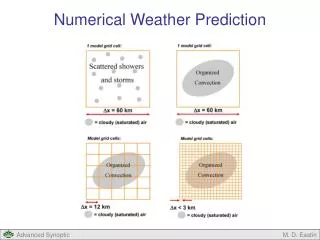
Developments in parameterizations of subgrid-scale processes • Parameterizations depend on horizontal resolution (examples: deep convection, microphysics) • Taking into account exchanges with adjacent horizontal grid cells (currenly, most of parameterizations are 1D in vertical)
New and advanced parameterizations of subgrid-scale processes • Advanced land surface parameterization accounting for hydrology, evolution of snow cover, freezing/melting, bogs, … • Deep convection parameterization for partially resolved case • Explicit description of microphysical processes in clouds • Lake parameterizations • Boundary layer parameterizations in the case of strongly stable stratification
Land surface parameterization «Tile» approach (subcells describing water, low and high vegetation, etc) New directions: • Soil hydrology taking into account adjacent grid cells • Biogeochemistry (carbon cycle, dynamical leaf area index …)
H-TESSEL surface parameterization scheme (ECMWF) The revised hydrology includes spatial variability related to topography (runoff) and soil texture (drainage) Slide 19
ECMWF: New microphysics parameterization WATER VAPOUR Evaporation Condensation CLOUD FRACTION CLOUD Liquid/Ice Evaporation CLOUD FRACTION Autoconversion PRECIP Rain/Snow Current Cloud Scheme New Cloud Scheme Slide 20
Data assimilation • Weight optimally observations and short-range forecast from previous initial conditions to create initial conditions for the model • Current approaches: 4D-Var and ensemble Kalman filter
Some directions of development for the global semi-Lagrangian model SL-AV • Increasing the scalability of the code from ~300 to 5000 processors • Replacement of 3D solvers by divide-and conquer algorithms • Nonhydrostatic dynamical core • More advanced land surface parameterization (bogs, carbon cycle, multilayer soil, soil hydrology…)
Conclusions • Challenges of the nearest decade – development and implementation of global atmospheric models with the horizontal resolution 1-10 km. • New approaches to develop new dynamical cores and parameterizations • This requires efficient parallel implementation on ~ 10000 processors ============================= We shorten the distance with leading centres in the field of global NWP