Download
1 / 35
350 likes | 385 Views
Understand the En-Var approach compared to 4D-Var and EnKF. Explore experimental results and operational systems in NWP. Learn the theory and practical applications of Sequential Data Assimilation Approach.

E N D
Data Assimilation for Numerical Weather Prediction: Current and Future Approaches Mark Buehner Meteorological Research Division, Environment Canada January 17, 2012 Air Quality Data Assimilation and Fusion Meeting Downsview, Ontario
Contents • Brief description of the data assimilation components of the Canadian operational NWP systems: 4D-Var, EnKF • The Ensemble-Variational (En-Var) approach and how it compares with 4D-Var and EnKF • Introduction to the project to modularize and then unify parts of the EnKF and variational assimilation codes • Experimental results from comparing En-Var with 4D-Var
Operational Data Assimilation Systems for global NWP • 4D-Var and EnKF: • both operational at CMC since 2005 • both use GEM forecast model • both assimilate similar set of observations using mostly the same observation operators and observation error covariances • 4D-Var is used to initialize medium range global deterministic forecasts (GDPS) • EnKF is used to initialize global Ensemble Prediction System (GEPS) • Starting in 2008, conducted a project to compare the EnKF and 4D-Var approaches, including various hybrid approaches • Project initiated in anticipation of WMO workshop on inter-comparison of 4D-Var and EnKF, Buenos Aires, November 2008
Operational Systems (as of January, 2012) • 4D-Var (Gauthier et al. 2007) • incremental approach: ~35km/150km grid spacing, 80 levels, 0.1hPa top • EnKF (Houtekamer and Mitchell 2005, Houtekamer et al. 2005) • 192 ensemble members: ~100km grid spacing, 58 levels, 2hPa top • uses 4D background-error covariances to produce 4D analysis (somewhat like 4D-Var, but without TL/AD of forecast model) • assimilates batches of observations sequentially by explicitly solving analysis equation and updating ensemble covariances • additive model and observation error perturbations and multiple physical parameterizations to simulate uncertainties
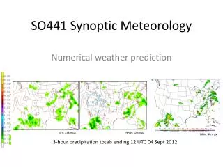
Example: CMC Deterministic Analysis and Forecasting System for NWP Data Assimilation:Goal is to correct a short-term forecast using information from all available observations
Sequential Data Assimilation Approach • Forecast and Analysis steps occur sequentially in time • Approach is well-suited for forecasting applications • Forecast step: • Using best estimate of current state, produce short-term forecast (usually 6h) with forecast model • Ideally, forecast should include uncertainty from errors in initial condition and forecast model • Analysis step: • Use all available observations to update forecast pdf and thus produce more accurate estimate of atmosphere state • Influence of observations governed by uncertainty from errors in the forecast and observations time t time t+1 time t+1 analysis (observations) forecast (model) var2 var2 var2 var1 var1 var1
Analysis Step: Theory • Bayes theorem is used to update pdf of forecast (x) using new set of observations (y) • Used to derive almost all data assimilation approaches • Differences among assimilation approaches result from particular choice of simplifying assumptions • In general, not feasible to work with full pdfs influence of observations background information independent of x (normalization)
Analysis Step: Theory • If all errors are Gaussian and unbiased the maximum likelihood estimate minimizes the function: • where: • xbis the short-term forecast used as the background state • B is the background error (forecast error) covariance matrix • y is the vector of observations • R is the observation error covariance matrix • Hmaps the analysis vector into observation space (obs operator): can include both spatial and temporal mapping (4D-Var) • Cis independent of x and therefore can be neglected
Analysis Step: Theory • If H() is linear, then the minimum of J(x) can be obtained by setting dJ/dx = 0 and solving for x, resulting in: • the Kalman filter and EnKF are based on solving this explicit equation for the analysis
Variational Data Assimilation • Iteratively seek the global minimum of cost function using a standard optimization algorithm (e.g. conjugate gradient or quasi-Newton), but stop after relatively few iterations: e.g. 50-100 • If obs operators (and forecast model for 4D-var) are linear, J is quadratic and possible to find unique minimum • Otherwise, obs operators (and forecast model for 4D-var) can be periodically re-linearized during minimization • In the case of nonlinearity, can be difficult to find the global minimum of a non-quadratic cost function linearized H and M J nonlinear H and M x local min global min
Different Flavours of Variational Assimilation + obs + + + 3D-Var + analysis + + ∆x + + + Background trajectory + + 3D-FGAT + + + + + + + + + + 4D-Var + + + + + + + + increment ∆x time
Ensemble Kalman Filter (EnKF) • The EnKF uses an ensemble of model integrations to explicitly propagate an approximation of the background and analysis error distributions • The background error covariances used to assimilate data are estimated from the background ensemble valid at the analysis time with little imposed constraints, except spatial localization: flow-dependent error covariances • The main sources of error in the analysis-forecast system are simulated by random perturbations (model error, observation error, forcing error) • Analysis ensemble supposed to represent a set of equally likely states: can be used to initialize an ensemble forecasts • Errors assumed to be Gaussian in formulation of analysis step, but not during forecast step!
Ensemble Kalman Filter (EnKF) • Approach is similar to the Extended Kalman Filter: • Forecast step for the mean: and the covariances: model error covariances M = linearized model • Analysis step for the mean: and the covariances: time t-1 time t time t analysis (observations) forecast (model) var2 var2 var2 var1 var1 var1
EnKF: Forecast step • For EnKF the means and covariance matrices of pdfs represented by relatively small (e.g. O(100)) random samples of the model state • Therefore, forecast step requires ~100 nonlinear model integrations: random model error realizations covariances required for analysis step: only uses nonlinear H()! analysis (observations) forecast (model) var2 var2 var2 var1 var1 var1
EnKF: Analysis step • For the analysis step, the observations are perturbed with random realizations of observation error, creating an ensemble of observations: • Then, a separate analysis is performed for each member using a different background state and set of perturbed observations drawn from their respective ensembles: Analysis uses ensemble-based background error covariances analysis (observations) forecast (model) var2 var2 var2 var1 var1 var1
EnKF: Analysis step, sequentially • Simultaneous assimilation of all observations not feasible due to required inversion of (HBHT+R) • Instead, sequentially assimilate batches of independent observations: Assimilate first batch of obs using background ensemble Assimilate second batch using analysis ensemble in place of background ensemble And so on for the m’th batch… assimilation of obs batch #1 assimilation of obs batch #2 etc. var2 var2 var2 var1 var1 var1
4D error covariancesTemporal covariance evolution (explicit vs. implicit evolution) EnKF (and En-Var): ensemble of NLM integrations 4D-Var: 55 TL/AD integrations, 2 outer loop iterations, then 3h NLM forecast -3h 0h +3h “analysis time”
Ensemble-Variational assimilation (En-Var) • Combine positive aspects of variational assimilation and the EnKF: • Iterative minimization of a cost function to assimilate all observations simultaneously (avoids sequential approach) • Use flow-dependent B matrix estimated from 4D ensemble of EnKF background states (avoids computational and development cost of TL/AD of GEM) • Allows ensemble B matrix to be combined with full-rank static B matrix currently used for 4D-Var (weighted average) and better spatial localization of covariances for non-local observations (e.g. radiances or total column ozone) • Better treatment of large volume of densely spaced observations • Like 3/4D-Var, can handle non-Gaussian cost function due to: e.g. Var-QC, observation operator • First goal is to produce a deterministic analysis that is competitive with current 4D-Var
Ensemble-Variational assimilation (En-Var) • Background-error covariances and analysed state are explicitly 4-dimensional, resulting in cost function: • 4D analysis is obtained without the use of TL/AD of forecast model (but TL/AD of obs operator still needed) • Computations involving B4D can be more expensive than with Bnmc depending on ensemble size and spatial resolution, but parallelization is possible
Strategy for modularization of variational assimilation system • started with v11.0.2 (recently upgraded to Strato2b-R version and introduced code required for GEM4) • original code is far too large to attempt a significant modularization • so, removed all code related to: regional analysis, singular vectors, psas, calculation of standard B matrix,… • removed most other code not required for global 3D-Var analysis (except recently reintroduced bgcheck code) • removed code related to several “modes” not currently being used: e.g. pressure level analysis, old formulation of B matrix • consolidated all setup in preproc.ftn (removed su0yoma/b, sucva) • once code is more modular, should be possible to introduce new functionality more easily: e.g. Regional/Yin-Yang En-Var • added functionality required for global En-Var (including hybrid covariances: B = (1-β) Bnmc + βBenkf ) • currently: number of comdecks: 75 21, fortran files: 837 212
Strategy for modularization of variational assimilation system • similar overall strategy as for EnKF • code is in SVN: “assimilation/glbvar” and “assimilation/shared” • frequent “commits” of code to minimize chance of introducing hard-to-find bugs • code updated in small, manageable increments • after each small increment, a short 3d-var minimization is run to ensure that results haven’t changed (rebm, anlm, brp*) • occasionally, change to code result in small change in results; requires special consideration – need to understand why results changed • unit tests and compilation are not yet automated, will be done in Maestro (Ervig) • initial goal is to test global En-Var as possible replacement of 4D-Var in GDPS – initial results are encouraging • ultimate goal is to start using modules that are shared with EnKF, but first requires high degree of modularity in each system
Modules completed or under construction(with help from Jeff) Low-level “data” modules: • ControlVector • GridStateVector(replaces comgd*) • ColumnData(replaces gomobs*) • ObsSpaceData(replaces CMA) • VerticalCoord • GaussGrid Transformational modules: • GlobalSpectralTransform • FFT (only used by GST) • BMatrixHI • BMatrixEnsemble • BMatrix Other modules: • Minimization • MPI • BUFR(bufr/burp constants) • MathPhysConstants Other code not yet in modules, but relying heavily on data modules: • Non-linear obs. operators • Linearized obs. operators • Obs. error statistics • brpacma, cmaabrp and sqlite I/O (P. Koclas)
Typical module contents Public contents (all public entities use common prefix, e.g. “obs_”): • derived type definition (i.e. the data part of the object) – eventually make all members of derived type private • subroutines/functions called by external code that require intimate knowledge of modules “details” (i.e. the module’s “interface”) Private contents: • namelist definition for parameters required by module (many modules have their own namelist) • module variables that are common to all “instances” of the object/class • subroutines/functions called only from within module Object/Class = derived type + module variable + all related subroutines/functions e.g. obsSpaceData – may create 1 or several “instances”, depending on application
Experimental Results • Tests with 3D-Var in the context of system with 58 levels, top at 10hPa (February 2008): • impact of using EnKF ensemble based covariances averaged with the NMC-based static covariances • Tests in the context of the currently operational GDPS using ensembles from previous version of EnKF with top at 10hPa and only 96 members (January-February 2011): • comparison of En-Var approach (with averaged covariances) relative to 4D-Var
Analysis and Forecast Verification Results Averaged covariances vs. Bnmc and Benkf(similar approach already operational at Met Office) Bavg = ½ Bnmc + ½ Benkf 3D-Var-Bavg vs. 3D-Var-Bnmc and 3D-Var-Bavg vs. 3D-Var-Benkf
Forecast Results:3D-Var-Bavg vs. 3D-Var-Bnmc north tropics south Difference in stddev relative to radiosondes: Positive 3D-Var-Bavg better Negative 3D-Var-Bnmc better zonal wind temp. height
Forecast Results:3D-Var-Bavg vs. 3D-Var-Benkf north tropics south Difference in stddev relative to radiosondes: Positive 3D-Var-Bavg better Negative 3D-Var-Benkf better zonal wind temp. height
Results – 500hPa GZ anomaly correlation Verifying analyses from 4D-Var with Bnmc Northern hemisphere Southern hemisphere Benkf0.50and0.75 are best Benkf0.75and 1.00 are best Bnmc and Benkf 1.00 worst Bnmc worst Bnmc Benkf 0.25 Benkf 0.50 Benkf 0.75 Benkf 1.00
Analysis and Forecast Verification Results En-Var vs. 3/4D-Var En-Var using averaged covariances: Bavg = [1-β(k)]Bnmc + β(k)Benkf with β=½ in troposphere, changing to β=0 at 10hPa (lid of EnKF) En-Var-Bavg vs. 3D-Var-Bnmc and En-Var-Bavg vs. 4D-Var-Bnmc
Forecast Results: 72h Forecasts vs RAOBSEn-Var-Bavg and 3D-Var-Bnmc northern extra-tropics southern extra-tropics
Forecast Results: 72h Forecasts vs RAOBSEn-Var-Bavg and 4D-Var-Bnmc northern extra-tropics southern extra-tropics
Forecast Results: 72h Forecasts vs ECMWFEn-Var-Bavg and 4D-Var-Bnmc north tropics south
Conclusions • En-Var approach is attractive possible alternative to 4D-Var and current EnKF sequential* analysis approach (*wrt batches of observations) • advantages of En-Var vs. full 4D-Var: • no need to maintain TL/AD version of model dynamics and physical parameterizations (EnKF members already available) • more computationally efficient and likely easier to parallelize for high spatial resolution and large data volumes • potential advantages from using En-Var within EnKF instead of current approach: • global analysis (all obs treated together – don’t have to perform all analyses in parallel, as with sequential batch approach) • localization of B instead of BHT (latter is a potential problem for non-local observations: satellite radiances) • allows use of alternative approaches for modelling covariances: e.g. averaged covariances • allows use of variational quality control (non-quadratic cost function)
Next Steps • Continue testing En-Var approach in current operational configuration of deterministic prediction system • use averaged covariances (with vertical level dependent weight) • redo tests in context of new versions of GDPS (25km resolution, GEM4), GEPS (~45km resolution, 192 members, GEM4) on Power 7 • test impact of introducing an outer loop • Examine possibility of using a variational approach for EnKF analysis step (computational cost of doing 192 En-Var minimizations!) • Continue to modularize/unify the code for Variational and EnKF data assimilation systems to facilitate further development of both systems and hybrid approaches
References Buehner, M., 2005, "Ensemble-derived stationary and flow-dependent background error covariances: Evaluation in a quasi-operational setting for NWP ." Quart. J. Roy. Meteor. Soc. Vol. 131, p1013-1044. Buehner, M., P.L. Houtekamer, C. Charette, H.L. Mitchell, B. He, 2010, "Intercomparison of variational data assimilation and the Ensemble Kalman Filter for global deterministic NWP. Part I: Description and Single-Observation experiments." Monthly Weather Review. Vol. 138, p1550-1566. Buehner, M., P.L. Houtekamer, C. Charette, H.L. Mitchell, B. He, 2010, "Intercomparison of variational data assimilation and the Ensemble Kalman Filter for global deterministic NWP. Part II: One-Month Experiments with Real Observations." Monthly Weather Review. Vol. 138, p1567-1586. Gauthier, P., M. Tanguay, S. Laroche, S. Pellerin, J. Morneau, 2007, “Extension of 3DVAR to 4DVAR: Implementation of 4DVAR at the Meteorological Service of Canada.” Mon. Wea. Rev., Vol 135, p2339–2354. Hamill, T. M. and Snyder, C. 2000 A hybrid ensemble Kalman filter—3D variational analysis scheme. Mon. Weather Rev., Vol. 128, p2905–2919. Hamill, T. M., Whitaker, J. S. and Snyder, C. 2001 Distance-dependent filtering of background error covariance estimates in an ensemble Kalman filter. Mon. Weather Rev., Vol. 129, p2776–2790 Houtekamer, P. L., H. L. Mitchell, G. Pellerin, M. Buehner, M. Charron, L. Spacek and B. Hansen, 2005, "Atmospheric data assimilation with the ensemble Kalman filter: Results with real observations ." Monthly Weather Review, Vol. 133, p604-620. Houtekamer, P. L., and H. L. Mitchell, 2005, “Ensemble Kalman filtering.” Quarterly Journal of the Royal Meteorological Society, Vol 131, p3269–3289 Houtekamer, P. L., H. L. Mitchell, X. Deng, 2009, “Model Error Representation in an Operational Ensemble Kalman Filter.” Monthly Weather Review. Vol 137, p2126-2143. Lorenc, A. C. 2003 The potential of the ensemble Kalman filter for NWP: A comparison with 4D-Var. Q. J. R. Meteorol. Soc., Vol. 129, p3183–3203.