Download
1 / 25
250 likes | 379 Views
CRaTER Thermal Analysis. Huade Tan 6/27/05. Contents. System Overview Requirements Inputs and Assumptions Power Dissipations Lunar Orbit Current Model Results Exterior instrument temperatures Orbital temperature ranges Performance Predictions Conclusions. System Overview.

E N D
CRaTER Thermal Analysis Huade Tan 6/27/05
Contents • System Overview • Requirements • Inputs and Assumptions • Power Dissipations • Lunar Orbit • Current Model • Results • Exterior instrument temperatures • Orbital temperature ranges • Performance Predictions • Conclusions
System Overview • Current Thermal System Requirements • Temperature Margin Philosophy • Hard/Survival limits define the range in which the instrument will not receive damage or permanent performance degredation • Qualification Limits are defined as the range of temperatures 10 degrees C wider than the flight predict limits • Flight Design limits define the range given by the current best estimates including margins of uncertainty in the given analysis. These limits must be within 10 degrees C of the hard limits. • Current Best Estimate ranges are determined by current state of testing and analysis • Requirement Exceedances • Current design does not exceed the given thermal requirements.
Inputs • Power Dissipations in the E-box • 200 mW distributed evenly throughout analog PCB • 2.1 W distributed evenly throughout digital PCB • Two power supplies, 1.2W and 0.9W mounted on digital PCB with a conductive resistance of Copper in a vacuum at 30 C • Power Dissipations in the telescope • 300 mW distributed evenly through three PCB’s, evenly stacked • Conduction characteristics modeled as wedge clamps along the sides of each board to the telescope housing.
MLI and Optical Bench • MLI outer layer optical properties: • Effective emittance: e* for MLI assumed to be .005 and .03 between best and worst cases. • CBE optical bench temperature margins between 16 and –19 C. • Modeled optical bench temperature margins between 35 and –30 C hot and cold.
Orbit • The current model is generated based on a basic Beta zero orbit at an altitude of 122.1 km. • This orbit was chosen in order to generate an orbital period of 7200 seconds. • Reducing the orbit to 50 km will shorten the orbital period and reduce the amplitude of resultant temperature fluctuations. • At a Beta angle of zero, the model simulates the worst case scenario where the instrument cycles from one temperature extreme to the other twice every period. • The total heat absorbed by the instrument through the given orbit is computed by the Radcad Monte Carlo method. • The model assumes a contact resistance of the mounting feet to LRO to be .5 W/cm2C. Radiation to the LRO is assumed to be through 15 layer MLI
Environmental Parameters • Orbital Heat Rate Factors: • Infrared Lunar Emissions are modeled after the temperature of the lunar surface. Lunar surface temperatures are modeled after the characteristic Lambertian surface having a subsolar temperature of 400 K and a shadow temperature of 100 K. • Surface temperatures across the bright side varies as a function of Tsubsolarcos1/4θ where θ is the angle measured from the orbital position to local noon. Brightness Temperatures of the Lunar Surface: The Clementine Long-Wave Infrared Global Data Set. Lawson SL and Jakosky BM.
Current Instrument Model • The reference coordinate system shown here is used to describe the exterior surfaces in the following slides • Where: • Xmax = left • Xmin = right • Ymax = front • Ymin = rear • Zmax = top • Zmin = bottom
Transient Results Summary • Current best estimates for CRaTER is primarily dependant upon the temperature margins given for the optical bench. • Instrument Interface temperatures vary +7 to –3 degrees C from the optical bench temperature between extremes of hot and cold. • Nine degrees C maximum temperature difference in instrument from mounting interface at the top cover (hot case). May consider an MLI outer layer with a lower absorbptivity.
Summary and Conclusions • Current Best Estimate: • Instrument interface temperature: 35 C 1 C Hot & -30C • Maximum instrument temperature exceeds no more that 2.6 degrees C from the interface temperature during orbit. • Uncertainties and Modeling Improvements: • Temperature dependence of material properties: Given a temperature fluctuation of a few degrees C through a beta 0 orbit, the temperature dependence of thermal properties can safely be neglected. • Incorporating TEPs into the thermal model • Finalizing mounting interface resistance to and relative view factors (to space) from the LRO • Incorporating actual circuitry details on the PCBs • Fine tuning MLI optical characteristics
Inputs • Thermal and Physical properties: • Optical Properties:
Assumptions • Material properties: • Thermophysical properties of Al-6061 obtained from Matweb databases • Optical properties of Aluminum obtained from Cooling Techniques for Electronic Equipment: Second Edition • MLI assumptions: • Currently modeled using bulk properties • PCB assumptions: • 2 ground and power layers (80% fill), 4 signal layers (20% fill), 1 mm thick • Properties determined at www.frigprim.com/online/cond_pcb.html • TEP assumptions: • Currently not modeled
Assumptions • Conductive Resistances: • Between PCB and Aluminum assumed to be characteristic of copper in vacuum at 30 C referred to in Heat Transfer. Holman, J.P • Within the Ebox assumed to be characteristic conduction of Al-6061 (assuming that the ebox is constructed out of a single block of aluminum) • Internal Radiation: • View factors of internal surfaces determined by Radcad using radk ray trace method • Emissivity factors calculated assuming either infinite parallel planes or general case for two surfaces from dissipating surfaces to interior walls. • Heat Flow to the Space Craft: • Assuming interface properties at 20 degrees C • Contact resistance of mounting feet to LRO assumed to be 20 W/cm2C • Radiation conduction to the LRO through 15 layer MLI
Current Telescope Model Note: the circular apertures on the top and bottom sides of the scope are insulated with a single layer of 3 mil black kapton