Download
1 / 5
50 likes | 288 Views
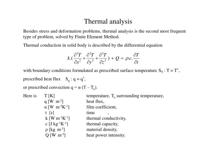
Thermal analysis Besides stress and deformation problems, thermal analysis is the second most frequent type of problem, solved by Finite Element Method. Thermal conduction in solid body is described by the differential equation

E N D
Thermal analysis Besides stress and deformation problems, thermal analysis is the second most frequent type of problem, solved by Finite Element Method. Thermal conduction in solid body is described by the differential equation with boundary conditions formulated as prescribed surface temperature ST : T = T*, prescribed heat flux Sq : q = q*, or prescribed convection q = α (T – To). Here is T [K] temperature, To surrounding temperature, q [W m-2] heat flux, α [W m-2K-1] film coefficient, t [s] time , k [W m-1K-1] thermal conductivity, c [J kg-1K-1] thermal capacity, ρ [kg m-3] material density, Q [W m-3] heat power intensity.
Appropriate functional, which is the basis of variational formulation of thermal conduction problem, has the form The primary unknown function is temperature, which is approximated in the same way as the displacements N is the matrix of shape functions and δTthe matrix of unknown nodal temperatures. The difference in comparison with displacements is, that temperature as scalar variable is fully described by a single value in node. For triangular element described in Chapter 4, the matrices are Time and space derivative of temperature are , where andL = .
Inserting this into the functional, we obtain for one finite element where k = ∫∫∫ BT.k. B dV element matrix of thermal conduction, c = ∫∫∫ NT..c.N dV element matrix thermal capacity and fQ = ∫∫∫ NT.QdV, fq = ∫∫ NT.q*dSq are matrices of thermal loading from internal and external sources. From the condition of stationary value of the functional of the whole body, completed from all elements in the same way as described in Chapter 2, we have the final form of discretised equation of thermal conduction where are global matrices of thermal capacity, conduction and loading and UT is the matrix of unknown nodal temperatures. The equation describes a non-stationary, transient problem of thermal conduction. As an illustrative example see the analysis of problem of temperature distribution in pipe-wall intersection in Example 10.1, its time evolution can be seen here.
Thermal stress analysis Many of machine parts are working at high temperatures. High temperature is the cause for thermal dilatation. Constraining this dilatation will lead to thermal stress. To analyse this phenomenon, we must divide the strain field into two components: stress and thermal strain The first one is caused by stress = D-1. , or = D . = D . ( - T ) . The second component is caused by thermal expansion T = .∆T = .[1,1,1,0,0,0]T. ∆T, where [K-1] is a thermal expansion coefficient. Inserting this into the strain energy expression, we can obtain the thermal expansion loading matrix, fT = ∫∫∫ BT. D. .∆TdV . which is used as a load matrix in a stress-displacement analysis. To formulate this matrix and compute thermal stress, a thermal analysis must be realised first so that we have the value of .∆Tin all nodes of the mesh. It is usual to run both analyses - thermal and stress - on the same mesh, changing only the type of element and analysis.
Corresponding element types in ANSYS are given in the Tab. 10.1. Illustration of the solution of coupled thermal-stress problem is given in the Example 4.3.