NUMERICAL ANALYSIS OF BIOLOGICAL AND ENVIRONMENTAL DATA

1. NUMERICAL ANALYSIS OF BIOLOGICAL AND ENVIRONMENTAL DATA Lecture 7. Direct Gradient Analysis

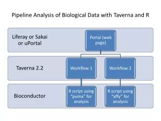
2. Interpretation of ordination axes with external data Canonical or constrained ordination techniques (= direct gradient analysis) DIRECT GRADIENT ANALYSIS Canonical correspondence analysis (CCA) Introduction Basic terms and ordination plots Other topics in CCA Robustness Scaling and interpretation of CCA plots Example Redundancy analysis (RDA) (= constrained PCA) Scaling and interpretation of RDA plots Statistical testing of constrained ordination axes Partial constrained ordinations Partial ordinations Partitioning variance Environmental (predictor) variables and their selection Canonical correlation analysis Distance-based redundancy analysis Canonical analysis of principal co-ordinates Principal response curves Polynomial RDA and CCA CCA/RDA as predictive tools Non-linear canonical analysis of principal co-ordinates Canonical Gaussian ordination Constrained additive ordination CANODRAW

3. BASIS OF CLASSICAL ORDINATION INTERPRETATION AND ENVIRONMENT We tend to assume that biological assemblages are controlled by environment, so: • Two sites close to each other in an indirect ordination are assumed to have similar composition, and • if two sites have similar composition, they are assumed to have similar environment. • In addition: • 3. Two sites far away from each other in ordination are assumed to have dissimilar composition, and thus • 4. if two sites have different composition, they are assumed to have different environment. J. Oksanen (2002)

4. DUNE-MEADOW DATA Values of environmental variables and Ellenberg’s indicator values of species written alongside the ordered data table of the Dune Meadow Data, in which species and sites are arranged in order of their scores on the second DCA axis. A1: thickness of A1 horizon (cm), 9 meaning 9cm or more; moisture: moistness in five classes from 1 = dry to 5 = wet; use: 1 = hayfield, 2 = a mixture of pasture and hayfield, 3 = pasture; manure: amount applied in five classes from 0 = no manure to 5 = heavy use of manure. The meadows are classified by type of management: SF, standard farming; BF, biological farming; HF, hobby farming; NM, nature management; F, R, N refer to Ellenberg’s indicator values for moisture, acidity and nutrients, respectively . Vegetational data Environmental data

5. DCA axis 2 DCA axis 1 The amount of manure written on the DCA ordination. The trend in the amount across the diagram is shown by an arrow, obtained by a multiple regression of manure on the site scores of the DCA axes. Also shown are the mean scores for the four types of management, which indicate, for example, that the nature reserves (NM) tend to lie at the top of the diagram. Ez=b0 + b1x1 + b2x2 Angle ()with axis 1 = arctan(b2 / b1)

6. Site scores of the second DCA axis plotted against the amount of manure.

7. Correlation coefficients (100  r) of the environmental variables for the four first DCA axes for the Dune Meadow Data Variable Axes   1 2 3 4 1 A1 58 24 7 9 2 moisture 76 57 7 -7 3 use 35 -21 -3 -5 4 manure 6 -68 -7 -64 5 SF 22 -29 5 -60 6 BF -28 -24 39 22 7 HF -22 -26 -55 -14 8 NM 21 73 17 56 Eigenvalue 0.54 0.29 0.08 0.05

8. Multiple regression of the first CA axis on four environmental variables of the dune meadow data, which shows that moisture contributes significantly to the explanation of the first axis, whereas the other variables do not. Term Parameter Estimate s.e. t constant c0 –2.32 0.50 –4.62 A1 c1 0.14 0.08 1.71 moisture c2 0.38 0.09 4.08 use c3 0.31 0.22 1.37 manure c4 –0.00 0.12 –0.01 ANOVA table d.f. s.s. m.s. F Regression 4 17.0 4.25 10,6 Residual 15 6.2 0.41 Total 19 23.2 1.22 R2 = 0.75 R2adj = 0.66 Ey1 = b0 + b1x1 + b2x2 + ...bnxn CA axis 1 environmental variables x = environmental variables

9. TWO-STEP APPROACH OF INDIRECT GRADIENT ANALYSIS Standard approach to about 1985: started by D.W. Goodall in 1954 Limitations: (1) environmental variables studied may turn out to be poorly related to the first few ordination axes. (2) may only be related to 'residual' minor directions of variation in species data. (3) remaining variation can be substantial, especially in large data sets with many zero values. (4) a strong relation of the environmental variables with, say, axis 5 or 6 can easily be overlooked and unnoticed. Limitations overcome by canonical or constrained ordination techniques = multivariate direct gradient analysis.

10. CANONICAL ORDINATION TECHNIQUES Ordination and regression in one technique – Cajo ter Braak 1986 Search for a weighted sum of environmental variables that fits the species best, i.e. that gives the maximum regression sum of squares Ordination diagram   1) patterns of variation in the species data   2) main relationships between species and each environmental variable Redundancy analysis  constrained or canonical PCA Canonical correspondence analysis (CCA)  constrained CA (Detrended CCA)  constrained DCA Axes constrained to be linear combinations of environmental variables. In effect PCA or CA with one extra step: Do a multiple regression of site scores on the environmental variables and take as new site scores the fitted values of this regression. Multivariate regression of Y on X.

11. Abundances or +/- variables Response variables Species Indirect GA Values Direct GA Predictor or explanatory variables Env. vars Classes PRIMARY DATA IN GRADIENT ANALYSIS PLUS

12. Artificial example of unimodal response curves of five species (A-E) with respect to standard-ised environmental variables showing different degrees of separation of the species curves moisture linear combination of moisture and phosphate CCA linear combination a: Moisture b: Linear combination of moisture and phosphate, chosen a priori c: Best linear combination of environmental variables, chosen by CCA. Sites are shown as dots, at y = 1 if Species D is present and at y = 0 if Species D is absent

13. Combinations of environmental variables e.g. 3 x moisture + 2 x phosphate e.g. all possible linear combinations zj = environmental variable at site j c = weights xj = resulting ‘compound’ environmental variable CCA selects linear combination of environmental variables that maximises dispersion of species scores, i.e. chooses the best weights (ci) of the environmental variables.

14. ALTERNATING REGRESSION ALGORITHMS - DCA - CCA - CA Algorithms for (A) Correspondence Analysis, (B) Detrended Correspondence Analysis, and (C) Canonical Correspondence Analysis, diagrammed as flowcharts. LC scores are the linear combination site scores, and WA scores are the weighted averaging scores.

15. REF REF CANONICAL CORRESPONDENCE ANALYSIS Algorithm 1) Start with arbitrary, but unequal, site scores xi. 2) Calculate species scores by weighted averaging of site scores. 3) Calculate new site scores by weighted averaging of species scores. [So far, two-way weighted average algorithm of correspondence analysis]. REF REF

16. REF REF 4) Obtain regression coefficients of site scores on the environmental variables by weighted multiple regression. where b and x* are column vectors Z is environmental data n x (q +1) R is n x n matrix with site totals in diagonal 5) Calculate new site scores or 6) Centre and standardise site scores so that: and 7) Stop on convergence, i.e. when site scores are sufficiently close to site scores of previous iteration. If not, go to 2. REF REF

17. CANONICAL OR CONSTRAINED CORRESPONDENCE ANALYSIS (CCA) • Ordinary correspondence analysis gives: • Site scores which may be regarded as reflecting the underlying gradients. • Species scores which may be regarded as the location of species optima in the space spanned by site scores. • Canonical or constrained correspondence analysis gives in addition: • 3. Environmental scores which define the gradient space. • These optimise the interpretability of the results. J. Oksanen (2002)

18. BASIC TERMS Eigenvalue = Maximised dispersion of species scores along axis. In CCA usually smaller than in CA. If not, constraints are not useful. Canonical coefficients = ‘Best’ weights or parameters of final regression. Multiple correlation of regression = Species–environment correlation. Correlation between site scores that are linear combinations of the environmental variables and site scores that are WA of species scores. Multiple correlation from the regression. Can be high even with poor models. Use with care! Species scores = WA optima of site scores, approximations to Gaussian optima along individual environmental gradients. Site scores = Linear combinations of environmental variables (‘fitted values’ of regression) (1). Can also be calculated as weighted averages of species scores that are themselves WA of site scores (2). (1) LC scores are predicted or fitted values of multiple regression with constraining predictor variables 'constraints'. (2) WA scores are weighted averages of species scores. Generally always use (1) unless all predictor variables are 1/0 variables.

19. SUMMARY OF DUNE MEADOW DATA Dune Meadow Data. Unordered table that contains 20 relevées (columns) and 30 species (rows). The right-hand column gives the abbreviation of the species names listed in the left-hand column; these abbreviations will be used throughout the book in other tables and figures. The species scores are according to the scale of van der Maarel (1979b).

20. Sample number A1 horizon Moisture class Management type Manure class Use 1 2.8 1 SF 2 4 2 3.5 1 BF 2 2 3 4.3 2 SF 2 4 4 4.2 2 SF 2 4 5 6.3 1 HF 1 2 6 4.3 1 HF 2 2 7 2.8 1 HF 3 3 8 4.5 5 HF 3 3 9 3.7 4 HF 1 1 10 3.3 2 BF 1 1 11 3.5 1 BF 3 1 12 5.8 4 SF 2 2* 13 6.0 5 SF 2 3 14 9.3 5 NM 3 0 15 11.5 5 NM 2 0 16 5.7 5 SF 3 3 17 4.0 2 NM 1 0 18 4.6* 1 NM 1 0 19 3.7 5 NM 1 0 20 3.5 5 NM 1 0 Environmental data of 20 relevées from the dune meadows Use categories: 1 = hay 2 = intermediate 3 = grazing * = mean value of variable

21. DCA DCA axis 2 DCA axis 1 DCA ordination diagram of the Dune Meadow Data

22. Axis Two 2 = 0.29 Axis One 1 = 0.54 DCA Correlations of environmental variables with DCA axes 1 and 2

23. CCA CCA of the Dune Meadow Data. a: Ordination diagram with environmental variables represented by arrows. the c scale applies to environmental variables, the u scale to species and sites. the types of management are also shown by closed squares at the centroids of the meadows of the corresponding types of management. 1 2 R axis 1 R axis 2 DCA 0.54 0.40 0.87 0.83 CCA 0.46 0.29 0.96 0.89

24. Variable Coefficients Correlations Axis 1 Axis 2 Axis 1 Axis 2 A1 9 -37 57 -17 Moisture 71 -29 93 -14 Use 25 5 21 -41 Manure -7 -27 -30 -79 SF - - 16 -70 BF -9 16 -37 15 HF 18 19 -36 -12 NM 20 92 56 76 CANONICAL CORRESPONDENCE ANALYSIS Canonical correspondence analysis: canonical coefficients (100 x c) and intra-set correlations (100 x r) of environmental variables with the first two axes of CCA for the Dune Meadow Data. The environmental variables were standardised first to make the canonical coefficients of different environmental variables comparable. The class SF of the nominal variable 'type of management' was used as a reference class in the analysis.

25. CCA of the Dune Meadow Data. a: Ordination diagram with environmental variables represented by arrows. the c scale applies to environmental variables, the u scale to species and sites. the types of management are also shown by closed squares at the centroids of the meadows of the corresponding types of management. a b b: Inferred ranking of the species along the variable amount of manure, based on the biplot interpretation of Part a of this figure.

26. BIPLOT PREDICTION OF ENVIRONMENTAL VARIABLES • Project a site point onto environmental arrow: predict its environmental value • Exact with two constraints only • Projections are exact only in the full multi-dimensional space. Often curved when projected onto a plane Modified from J. Oksanen (2002)

27. REF REF CLASS VARIABLES • Class 1/0 variables usually represented as 'dummy' variables: make m - 1 indicator variables out of m levels (moisture classes 1, 2, 4, 5). Ignore class 3 • Scoring: 1 if site belongs to the class, 0 otherwise • One dummy less than levels, because one is redundant. If it does not belong to any of the m - 1 classes, it must belong to the remaining one. • Ordered factors such as the four moisture classes can be expressed as polynomial constraints. A four-level ordered factor can be expressed in three 'dummy' variables - linear, quadratic, and cubic effects. Plot as biplot arrows. Helps to find when one can replace a multilevel factor by a single continuous variable (e.g. Moisture Linear) J. Oksanen (2002) REF

28. CCA: JOINT PLOTS AND TRIPLOTS • You may have in a same figure • WA scores of species • WA or LC scores of sites • Biplot arrows or class centroids of environmental variables • In full space, the length of an environmental vector is 1: When projected onto ordination space • Length tells the strength of the variable • Direction shows the gradient • For every arrow, there is an equal arrow to the opposite direction, decreasing direction of the gradient • Project sample points onto a biplot arrow to get the expected value • Class variables coded as dummy variables • Plotted as class centroids • Class centroids are weighted averages  • LC score shows the class centroid, WA scores show the dispersion of the centroid • With class variables only: Multiple Correspondence Analysis or Analysis of Concentration

29. CANOCO Summary Axes Axes 1 2 3 4 Total inertia Eigenvalues .461 .298 .160 .134 2.115 Species-environment .958 .902 .855 .889 correlations Cumulative percentage variance of species data 21.8 35.9 43.5 49.8 of species-environment 37.8 62.3 75.4 86.3 relation Sum of all unconstrained eigenvalues = inertia 2.115 Sum of all canonical eigenvalues = species-environment 1.220 relation 'Fitted' species data Rules of thumb: >0.30 strong gradient >0.40 good niche separation of species

30. CONVERGENCE CRITERIA IN EIGENVALUE EXTRACTION Oksanen & Minchin (1997) J. Vegetation Science 8, 447–454 Tolerance Number of iterations DECORANA 0.0001 10 CANOCO version 2 0.00005 15 version 3.1 CANOCO version 3.12a 0.000005 999 (‘STRICT’ CRITERIA) CANOCO version 4 0.000005 999

31. OTHER CCA TOPICS 1) Environmental variables   continuous – biplot arrows classes – centroid (weighted average) of sites belonging to that class 2) CA approximates ML solution of Gaussian model CCA approximates ML solution of Gaussian model if CA axis is close to the linear com-bination of environmental variables. [Johnson & Altman (1999) Environmetrics 10, 39-52] In CCA species compositional data are explained through a Gaussian unimodal response model in which the explanatory variable is a linear combination of environmental variables. 3) CCA – very robust, major assumption is that response model is UNIMODAL. (Tolerances, maxima, and location of optima can be violated - see Johnson & Altman 1999) 4) Constraints become less and less strict the more environmental variables there are. If q, number of environmental variables ≥ number of samples -1, no real constraints and CCA = CA. 5) Arch effect may crop up. Detrending (by polynomials) DCCA. Useful for estimating gradient lengths (use segments). 6) Arch effect can often be removed by dropping superfluous environmental variables, especially those highly correlated with the arched axis.

32. REPRESENTATION OF CLASS VARIABLES (1/0) IN CCA • Make class centroids as distinct as possible • Make clouds about centroids as compact as possible • Success   • LC scores are the class centroids: the expected locations, WA scores are the dispersion of the centroid • If high , WA scores are close to LC scores • With several class variables, or together with continuous variables, the simple structure can become blurred J. Oksanen (2002)

33. Canonical correspondence analysis Unimodal curves for the expected abundance response (y) of four species against an environmental gradient or variable (x). The optima, estimated by weighted averages, (u) [k=1,2,3], of three species are indicated. The curve for the species on the left is truncated and therefore appears monotonic instead of unimodal; its optimum is outside the sampled interval but, its weighted average is inside. The curves drawn are symmetric, but this is no strict requirement for CCA.

34. 7) t-values of canonical coefficients or forward selection option in CANOCO to find minimal set of significant variables that explain data about as well as full set. 8) Can be sensitive to deviant sites, but only if there are outliers in terms of both species composition and environment. CCA usually much more robust than CA. 9) Can regard CCA as a display of the main patterns in weighted averages of each species with respect to the environmental variables.   Intermediate between CA and separate WA regressions for each species.   Separate WA regressions  point in q-dimensional space of environmental variables. NICHE.   CCA attempts to provide a low-dimensional representation of this niche. 10) ‘Dummy’ variables (e.g. group membership or classes) as environmental variables. Shows maximum separation between pre-defined groups. 11) ‘Passive’ species or samples or environmental variables. Some environmental variables active, others passive   e.g. group membership – active environmental variables – passive 12) CANOCO ordination diagnostics   fit of species and samples pointwise goodness of fit can be expressed either as residual distance from the ordination axis or plane, or as proportion of projection from the total chi-squared distance species tolerances, sample heterogeneity

35. Passive ‘fossil’ samples added into CCA of modern data

36. Canonical correspondence analysis (CCA) time-tracks of selected cores from the Round Loch of Glenhead; (a) K5, (b) K2, (c) K16, (d) k86, (e) K6, (f) environmental variables. Cores are presented in order of decreasing sediment accumulation rate.

37. 13) Indicator species 14) Behaves well with simulated data. M W Palmer (1993) Ecology 74, 2215–2230 Copes with skewed species distributions ‘noise’ in species abundance data unequal sampling designs highly intercorrelated environmental variables situations when not all environmental factors are known

38. Site scores along the first two axes in CCA and DCA ordinations, with varying levels of quantitative noise in species abundance. Quantitative noise was not simulated. The top set represents CCA LC scores and environmental arrows, the middle represents CCA WA scores, and the bottom represents DCA scores. Sites with equal positions along the environmental gradient 2 are connected with lines to facilitate comparisons. Palmer, M.W. (1993) Ecology 74, 2215–2230

39. ..continued Site scores along the first two axes in CCA and DCA ordinations, with varying levels of quantitative noise in species abundance. Quantitative noise was not simulated. The top set represents CCA LC scores and environmental arrows, the middle represents CCA WA scores, and the bottom represents DCA scores. Sites with equal positions along the environmental gradient 2 are connected with lines to facilitate comparisons. Palmer, M.W. (1993) Ecology 74, 2215–2230

40. ROBUSTNESS OF CANONICAL CORRESPONDENCE ANALYSIS Like all numerical techniques, CCA makes certain assumptions, most particularly that the abundance of a species is a unimodal function of position along environmental gradient. Does not have to be symmetric unimodal function. Simulated data Palmer 1993 – CCA performs well even with highly skewed species distributions. ‘Noise’ in ecological data – errors in data collection, chance variation, site-specific factors, etc. Noise is also regarded as ‘unexplained’ or ‘residual’ variance. Regardless of cause, noise does not affect seriously CCA. ‘Noise’ in environmental data is another matter. In regression, assumed that predictor variables are measured without error. CCA is a form of regression, so noise in environmental variables can affect CCA. Highly correlated environmental variables, e.g. soil pH and Ca. Species distributions along Ca gradient may be identical to distributions along pH gradient, even if one is ecologically unimportant. Species and object arrangement in CCA plot not upset by strong inter-correlations. CCA (like all other regression techniques) cannot tell us which is the ‘real’ important variable. Both may be statistically significant – small amount of variation in Ca at a fixed level of pH may cause differences in species composition. Arch – very rarely occurs in CCA. Detrended CCA generally should not be used except in special cases.

41. INFLUENCE OF NOISY ENVIRONMENTAL DATA ON CANONICAL CORRESPONDENCE ANALYSIS McCune (1997) Ecology 78, 2617–2623 Simulated artificial data 10 x 10 grid. 40 species following Gaussian response model. (1) (2) (3) (4) (5) • 2 environmental variables X and Y co-ordinates TENXTEN • 2 environmental variables with added noise NOISMOD • (random number mean = 0, variance 17%) • added to each cell • 10 random environmental variables NOIS1O • 2 environmental variables with added noise from NOISMOD • + • random environmental variables from NOIS 10 • NOISBOTH • 99 random environmental variables NOISFULL NOISFULL – ‘Species-environment’ correlation increases as number of random variables increases for axis 1 and 2. Is in fact the correlation between the linear combination and WA site scores. Poor criterion for evaluating success. Not interpreted as measure of strength of relationship. Monte Carlo permutation tests - NO STATISTICAL SIGNIFICANCE!

42. TEN x TEN NOISMOD NOISIO Dependence of the 'species-environment correlation,' the correlation between the LC and WA site scores, on a second matrix composed of from 1 to 99 random environmental variables. This correlation coefficient is inversely related to the degree of statistical constraint exerted by the environmental variables. NOISFULL

43. Monte Carlo tests 12r1r2 TENXTEN * 0.77 0.79 0.98 0.9 NOISMOD * 0.65 0.65 0.90 0.8 NOISE 10 ns 0.20 0.12 0.49 0.4 NOISBOTH * 0.65 0.65 0.91 0.8 NOISFULL ns 0.12 0.08 1.0 1.0 (99 env vars) Linear combination site best fit of species abundances to scores the environmental data WA site scores best represent the assemblage structure ‘Species-environmental correlation’ better called ‘LC-WA’ correlation. Better measure of the strength of the relationship is the proportion of the variance in the species data that is explained by the environmental data. Evaluation should always be by a Monte Carlo permutation test. LC scoresWA scores Sensitive to noise +– True direct gradient analysis +– (multivariate regression) Aim to describe biological +– variation in relation to environment Assemblage structure –+ Which to use depends on one's aims and the nature of the data.

44. LC OR WA SCORES? MIKE PALMER "Use LC scores, because they give the best fit with the environment and WA scores are a step from CCA towards CA." BRUCE MCCUNE "LC scores are excellent, if you have no error in constraining variables. Even with small error, LC scores can become poor, but WA scores can be good even in noisy data." LC scores are the default in CANODRAW. Be aware of both - plot both to be sure. J. Oksanen (2002)

45. DATA ORDERINGS

46. CCA DIAGRAM TEN SETS OF DISTANCES TO REPRESENT, EMPHASIS ON 5, 8, AND 1 (FITTED ABUNDANCES OF SPECIES AND SITES)

47. Data-tables in an ecological study on species environmental relations. Primary data are the sub-table 1 of abundance values of species and the sub-tables 4 and 7 of values and class labels of quantitative and qualitative environmental variables (env. var), respectively. The primary data are input for canonical correspondence analysis (CCA). The other sub-tables contain derived (secondary) data, as the arrows indicate, named after the (dis)similarity coefficient they contain. The coefficients shown in the figure are optimal when species-environmental relations are unimodal. The CA ordination diagram represents these sub-tables, with emphasis on sub-tables 5 (weighted averages of species with respect to quantitative environmental variables), 8 (totals of species in classes of qualitative environmental variables) and 1 (with fitted, as opposed to observed, abundance values of species). The sub-tables 6, 9, and 10 contain correlations among quantitative environmental variables, means of the quantitative environmental variables in each of the classes of the qualitative variables and chi-square distances among the classes, respectively. (Chis-sq = Chi-square; Aver = Averages; Rel = Relative)

48. DEFAULT CCA PLOT • Like CA biplot, but now a triplot: vectors for linear constraints. • Classes as weighted averages or centroids. • Most use LC scores: these are the fitted values. • Popular to scale species relative to eigenvalues, but keep sites unscaled. Species-conditional plot. • Sites do not display their real configuration, but their projections onto environmental vectors are the estimated values. J. Oksanen (2002)

49. fitted by least squares REF REF SCALING IN CCA Hill scaling Default scaling –1 2 Emphasis on SITES SPECIES 1 Species x sites Rel abundances Fitted abundances (rel) 2 Species x species – Chi-squared distances 3 Sites x sites Turnover distances – Quant env vars 4 Sites x env vars3 – Values of env vars 5 Species x env vars Weighted averages Weighted averages 6 Env vars x env vars Effects2 Correlations2 Qualit env vars 7 Sites x env classes4 Membership1 Membership1 8 Species x env classes Rel total abund Rel total abund 9 Env vars x env classes – Mean values of env vars 10 Env classes x env Turnover distances – classes 1 by centroid principle 2 change in site scores if env variable changes are one standard deviation 3 inter-set correlations 4 group centroids REF REF

50. REF REF Sub-tables (row numbers) that can be displayed by two differently scaled ordination diagrams in canonical correspondence analysis (CCA). Display is by the biplot rule unless noted otherwise. Hill's scaling (column 2) was the default in CANOCO 2.1, whereas the species-conditional biplot scaling (column 3) is the default in CANOCO 3.1 and 4. The weighted sum of squares of sites scores of an axis is equal to /(1-) with  its eigenvalue and equal to 1 in scaling -1 and scaling 2, respectively. The weighted sum of squares of species scores of an axis is equal to 1/(1-) and equal to  in scaling -1 and scaling 2, respectively. If the scale unit is the same of both species and sites scores, then sites are weighted averages of species scores in scaling -1 and species are weighted averages of site scores in scaling 2. Table in italics are fitted by weighted least-squares (rel. = relative; env. = environmental; cl. = classes; - = interpretation unknown). Note that symmetric scaling (=3) has many optimal properties (Gabriel, 2002; ter Braak, personal communication) REF REF