Download
1 / 58
650 likes | 1.04k Views
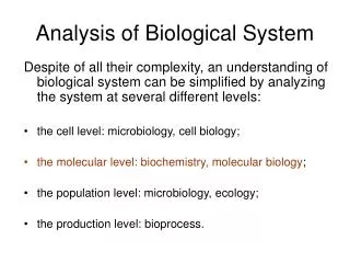
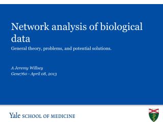
Network analysis of biological data. A Jeremy Willsey Gene760 - April 08, 2013. General theory, problems, and potential solutions. Overview. Goal of network analysis Types of biological networks Network analysis concepts Properties of biological networks

E N D
Network analysis of biological data A Jeremy Willsey Gene760 - April 08, 2013 General theory, problems, and potential solutions.
Overview • Goal of network analysis • Types of biological networks • Network analysis concepts • Properties of biological networks • Issues with ‘conventional’ (database-reliant) network analysis • Co-expression analysis – general concepts & implementation • Co-expression analysis – WGCNA • Successful applications of WGCNA • Pitfalls of co-expression analysis • Appendix: Network analysis tools and software
Network analysis converts biological information into network structure • The goal of network analysis is to connect genes or proteins meaningfully in order to elucidate the underlying biology • Actionable understanding of gene-gene or protein-protein relationships • Identification of key genes • Network analysis is becoming common in biology • Explosion of publicly available biological data • Biological activities depend on coordinated effects of many interacting species, the study of these interactions is fundamental to understanding biological systems • Understanding the complexity of most human diseases requires pathway level knowledge • Developments in systems biology network theory (i.e. ubiquity of scale free topology) A.-L. Barabási, N. Gulbahce, J. Loscalzo, Network medicine: a network-based approach to human disease, Nat Rev Genet12, 56–68 (2011).
Types of biological networks • Protein-protein interaction networks • Yeast two-hybrid • Immunoprecipitation and high-throughput mass-spectrometry • Individually validated interactions (mined from databases) • Predicted function (orthology, paralogy) • Text mining • Metabolic networks • System of connected enzymatic/chemical reactions • Generally very well characterized • Regulatory networks • ChIP-on-chip • ChIP-seq • RNA networks • RNA-RNA and RNA-DNA interactions • Gene co-expression networks • Patterns of gene expression connect genes A.-L. Barabási, N. Gulbahce, J. Loscalzo, Network medicine: a network-based approach to human disease, Nat Rev Genet12, 56–68 (2011).
Networks are composed of nodes and edges (connections between nodes) • In biological networks (graphs), nodes (vertices) typically represent genes, proteins, or metabolites whereas edges represent relationships • Formally, a graph G can be defined as a pair (V,E) where V is a set of vertices representing the nodes and E is a set of edges representing the connections between the nodes • Define as E= {(i,j) | i, j, εV} the single connection between nodes (i.e. E=(1,2) ) • Graph can be represented as a symmetric adjacency matrix made of 0’s and 1’s where 1 represents a connection between two nodes which are the rows and columns Corresponding adjacency matrix Nodes 2 3 Hub 1 4 5 Edges G. A. Pavlopouloset al., Using graph theory to analyze biological networks, BioData Mining4, 10 (2011).
Networks can be undirected, directed, or weighted Undirected • Edges represent biological relationships • Multi-edge connections are possible, used to represent multiple relationships 2 3 1 4 5 G. A. Pavlopouloset al., Using graph theory to analyze biological networks, BioData Mining4, 10 (2011).
Networks can be undirected, directed, or weighted Undirected Corresponding adjacency matrix 2 3 1 4 5 G. A. Pavlopouloset al., Using graph theory to analyze biological networks, BioData Mining4, 10 (2011).
Example: PPI database String (http://string-db.org/) - evidence view • Edges represent associations based on several forms of evidence Different colors represent different types of evidence for association
Networks can be undirected, directed, or weighted Directed • Edges retain directionality • Commonly used for metabolic, signal transduction, or regulatory networks 2 3 1 4 5 G. A. Pavlopouloset al., Using graph theory to analyze biological networks, BioData Mining4, 10 (2011).
Networks can be undirected, directed, or weighted Directed Corresponding adjacency matrix 2 3 1 4 5 G. A. Pavlopouloset al., Using graph theory to analyze biological networks, BioData Mining4, 10 (2011).
Example: PPI database String (http://string-db.org/) - action view • Edges represent connection and type of relationship Modes of action are shown in different colors
Example: KEGG http://www.genome.jp/kegg/ • Edges represent activating or inhibiting interactions
Networks can be undirected, directed, or weighted Weighted • Most widely used type of network in bioinformatics • Weight of edge indicates strength of connection (or confidence, relevance, etc) 2 3 1 4 5 G. A. Pavlopouloset al., Using graph theory to analyze biological networks, BioData Mining4, 10 (2011).
Networks can be undirected, directed, or weighted Weighted Corresponding adjacency matrix 2 3 1 4 5 G. A. Pavlopouloset al., Using graph theory to analyze biological networks, BioData Mining4, 10 (2011).
Example: PPI database String (http://string-db.org/) - confidence view • Edges represent strength of association (based on strength of evidence) Stronger associations are represented by thicker lines
Properties of biological networks • Biological networks tend to follow a series of basic organizing principles that distinguish them from random networks • Modules • Highly interlinked (connected) local regions in the network • Degree distribution and hubs – scale free topology • Degree distribution (fraction of nodes with a given degree) decays according to a power law (as opposed to Poisson distribution) • Afew highly connected genes (hubs) hold the networks together • Small world phenomena • Short path between any pair of nodes • Motifs • Subgraphs repeated within or across multiple networks • Betweenness centrality • Some genes mediate connections between subnetworks A.-L. Barabási, N. Gulbahce, J. Loscalzo, Network medicine: a network-based approach to human disease, Nat Rev Genet12, 56–68 (2011).
What do these properties mean for biological network analysis? • Modules • Correspond to ‘functional’ units • Degree distribution and hubs – scale free topology • Some genes (hubs) contribute more to network structure, these are likely more important • Small world phenomena • Perturbing the state of a given node can perturb other nodes and have consequences for the entire network • Motifs • Likely associated with optimized biological function (i.e. negative feedback) • Betweenness centrality • Nodes with high betweenness centrality tend to correlate with essentiality A.-L. Barabási, N. Gulbahce, J. Loscalzo, Network medicine: a network-based approach to human disease, Nat Rev Genet12, 56–68 (2011).
Conventional network analysis is fraught with problems • Databases are incomplete • Some data is incorrect • Investigative biases • Annotation biases • Inability to determine novel relationships • Lack of spatiotemporal consideration • Which databases to use? Which tools/methods to use? • Consistency / reproducibility across methods http://clair.si.umich.edu/~radev/cs6998/papers_to_replicate/nbt0108-69.pdf
GeneMANIAhttp://genemania.org/ String (http://string-db.org/) • Both methods use the same general set of databases • 2/10 String network nodes are found in the GeneMANIAnetwork • Different methods of weighting evidence
Building networks from expression data • Genes with similar co-expression patterns are connected • Hypotheses: • Co-expressed genes function together • Co-expressed genes are likely co-regulated • Overcomes many of the aforementioned issues with network analysis • Does not rely on divergent or heterogenousdatabases • Ability to determine novel relationships • Spatiotemporal information utilized • Methods for determining co-expression networks are relatively simple, well established, and consistent (Pearson’s correlation)
Co-expression analysis seeks to group genes based on similarity of expression profiles • Determine pairwise correlations between genes across a set of samples • Connect genes with similar expression profiles (co-expressed genes) • Group sets of highly connected genes P. Langfelder, S. Horvath, WGCNA: an R package for weighted correlation network analysis, BMC Bioinformatics9, 559 (2008).
Co-expression analysis seeks to group genes based on similarity of expression profiles • Determine pairwise correlations between genes across a set of samples • Connect genes with similar expression profiles (co-expressed genes) • Group sets of highly connected genes P. Langfelder, S. Horvath, WGCNA: an R package for weighted correlation network analysis, BMC Bioinformatics9, 559 (2008).
Co-expression analysis can be bottom-up or top-down • Bottom-up approach • Co-expressed genes are connected and grouped together by interconnectedness (unsupervised clustering) • Determine global system structure, emergent properties of the data • Useful for hypothesis-naïve approach to network construction • Top-down approach • Start with a set of ‘seed’ genes and build outwards to determine local system • Useful for hypothesis-driven approach to network construction
Weighted gene co-expression network analysis (WGCNA) P. Langfelder, S. Horvath, WGCNA: an R package for weighted correlation network analysis, BMC Bioinformatics9, 559 (2008).
WGCNA – Step 1 Network Construction • Define n x m matrix X = [xil] where the row indices correspond to genes (nodes, i= 1, …, n) and the column indices (l = 1, …, m) correspond to sample measurements Matrix X of expression level Node profile P. Langfelder, S. Horvath, WGCNA: an R package for weighted correlation network analysis, BMC Bioinformatics9, 559 (2008).
WGCNA – Step 1 Network Construction • Define n x m matrix X = [xil] where the row indices correspond to genes (nodes, i= 1, …, n) and the column indices (l = 1, …, m) correspond to sample measurements • Correlation network methodology describes pairwise relationships (correlations) between the rows of X Matrix X of expression level Node profile Positively correlated P. Langfelder, S. Horvath, WGCNA: an R package for weighted correlation network analysis, BMC Bioinformatics9, 559 (2008).
WGCNA – Step 1 Network Construction • Define n x m matrix X = [xil] where the row indices correspond to genes (nodes, i= 1, …, n) and the column indices (l = 1, …, m) correspond to sample measurements • Correlation network methodology describes pairwise relationships (correlations) between the rows of X Matrix X of expression level Node profile Negatively correlated P. Langfelder, S. Horvath, WGCNA: an R package for weighted correlation network analysis, BMC Bioinformatics9, 559 (2008).
WGCNA – Step 1 Network Construction • Define n x m matrix X = [xil] where the row indices correspond to genes (nodes, i= 1, …, n) and the column indices (l = 1, …, m) correspond to sample measurements • Correlation network methodology describes pairwise relationships (correlations) between the rows of X Matrix X of expression level Node profile Not correlated P. Langfelder, S. Horvath, WGCNA: an R package for weighted correlation network analysis, BMC Bioinformatics9, 559 (2008).
WGCNA – Step 1 Network Construction • Define co-expression similarity sij between genes i and j as • sij = |cor(xi,xj)| • i.es1,2 = -0.98s1,3 = 1.00s1,n = -0.06 Matrix X of expression level Node profile P. Langfelder, S. Horvath, WGCNA: an R package for weighted correlation network analysis, BMC Bioinformatics9, 559 (2008).
WGCNA – Step 1 Network Construction - unweighted Unweighted adjacency matrix • Define co-expression similarity sij between genes i and j as • sij = |cor(xi,xj)| • Create adjacency matrix aij from all s • Unweighted 1 if sij ≥ τ 0 otherwise aij= P. Langfelder, S. Horvath, WGCNA: an R package for weighted correlation network analysis, BMC Bioinformatics9, 559 (2008).
WGCNA – Step 1 Network Construction - weighted Weighted adjacency matrix • Define co-expression similarity sij between genes i and j as • sij = |cor(xi,xj)| • Create adjacency matrix aij from all s • Unweighted 1 if sij ≥ τ 0 otherwise • Weighted[aij] = [sij]ORaij = sijβ aij= Choose βas lowest power for which the scale free fit index ≥0.90 P. Langfelder, S. Horvath, WGCNA: an R package for weighted correlation network analysis, BMC Bioinformatics9, 559 (2008).
WGCNA – Step 2 Module Detection • Define modules as clusters of densely connected genes • Determine network interconnectedness using topological overlap measure (TOM) • A pair of nodes has high topological overlap if they are strongly connected to the same group of nodes • In gene networks, genes with high topological overlap are likely to be in the same biological pathway Low topological overlap High topological overlap P. Langfelder, S. Horvath, WGCNA: an R package for weighted correlation network analysis, BMC Bioinformatics9, 559 (2008).
WGCNA – Step 2 Module Detection • Convert TOM to dissimilarity measure (1-TOM) & identify modules using unsupervised hierarchical clustering and branch cutting algorithm • Modules correspond to sets of rows of X that are highly correlated (low dissimilarity measure) Weighted adjacency matrix Module P. Langfelder, S. Horvath, WGCNA: an R package for weighted correlation network analysis, BMC Bioinformatics9, 559 (2008).
WGCNA – Step 3 Relate modules to external data and identify important genes • Define sample trait T as a vector with m components (T = (T1, … Tm) that correspond to the columns (samples) of the matrix X • Trait-based node significance (GSi) measure can be defined as • GSi = |cor(xi, T)| • We can prioritize genes by significance measure and modules by average gene significance measure P. Langfelder, S. Horvath, WGCNA: an R package for weighted correlation network analysis, BMC Bioinformatics9, 559 (2008).
WGCNA – Step 3 Relate modules to external data and identify important genes • Define sample trait T as a vector with m components (T = (T1, … Tm) that correspond to the columns (samples) of the matrix X • Trait-based node significance (GSi) measure can be defined as • GSi = |cor(xi, T)| • We can prioritize genes by significance measure and modules by average gene significance measure • Can also examine gene ontology enrichment, burden of disease loci (GWAS, known mutations, etc) P. Langfelder, S. Horvath, WGCNA: an R package for weighted correlation network analysis, BMC Bioinformatics9, 559 (2008).
WGCNA – Step 4 Study module relationships • Define the module eigengeneE as the first principal component of a given module • Considered representative of the gene expression profiles in a module • Rationale is to understand how modules interact; also reduction in data, multiple comparisons P. Langfelder, S. Horvath, WGCNA: an R package for weighted correlation network analysis, BMC Bioinformatics9, 559 (2008).
Clustering of eigengenes identifies meta-modules and trait associations
WGCNA – Step 5 Identify key drivers in interesting modules • Output from Steps 1-4 • Candidate modules • Candidate genes within these modules • Need hypothesis-driven experimental validation • Additional clinical data or follow up in patients • Targeted sequencing of candidate genes • Perturbation of key genes (hubs) in human cell lines or model organisms • Build networks with alternative methods and data and examine convergence P. Langfelder, S. Horvath, WGCNA: an R package for weighted correlation network analysis, BMC Bioinformatics9, 559 (2008).
WGCNA Example 1 Nature478, 483–489 (2011).
The dataset is a comprehensive map of gene expression patterns in the developing human brain • Whole transcriptome profiling across 1,340 tissue samples collected from 57 developing and adult post-mortem brains of clinically unremarkable donors (males & females of multiple ethnicities) • Samples from transient prenatal structures and immature and mature forms of 16 brain regions (11 neocortical, 5 non-neocortical) from each sample • N=57 (39 with both hemispheres) • Age: 5.7 weeks post-conception to 82 years • Sex: 31 males and 26 females • Post-mortem interval 12.11 ± 8.63hours • pH 6.45 ± 0.34 • Total RNA extracted from each sample (RIN 8.83 ± 0.93) • Gene expression assessed with the AffymetrixGeneChip Human Exon 1.0 ST Array platform • Comprehensive coverage of the human genome, 1.4 million probe sets assaying expression across entire transcripts and individual exons Kang, H. J. et al.Spatio-temporal transcriptome of the human brain. Nature478, 483–489 (2011).
WGCNA performed on the multidimensional spatio-temporal dataset identified 29 modules • General quality control • No large-scale structural abnormalities identified by genotyping • Hierarchical clustering • Remove outliers and nsure clustering by region and time, not by covariates • Averaged Spearman correlation coefficient of a given brain region / NCX area calculated for each period • Remove outliers • WGCNA Data cleaning steps: • Brain-expressed genes only: log2(intensity) > 6 in at least 1 sample • Coefficient of variance > 0.08 • Total of 9,093 genes fit this criteria
Module M8 may be important for development of neocortical and hippocampal projection neurons Hub genesinclude transcription factors TBR1, FEZF2, FOXG1, SATB2, NEUROD6 and EMX1 - functionally implicated in the development of NCX and HIP projection FOXG1 variants have also been linked to Rett syndrome and intellectual disability • 24 Genes • Gene ontology enrichment: • Neuronal differentiation p* = 0.008 • Transcription factors p* = 0.005*Bonferroni-adjusted
Module M15 may be important for neurotransmission • 310 Genes • Gene ontology enrichment: • Ionic channels p* = 8.0 x10⁻⁸ • Neuroactive ligand-receptor interaction p* = 4.0 x10⁻¹⁴*Bonferroni-adjusted Sequence variants in Hub genesare linked to major depression (GDA) and to schizophrenia and affective disorders (NRGN andRGS4)
Modules M20 and M2 have opposite trajectories and drastic changes near birth Module M2 Module M20 • GO enrichment for • membrane proteins (P = 1.8 × 10⁻²¹) • calcium signalling (P = 8.1 × 10⁻¹⁰), • synaptic transmission (P = 1.6 × 10⁻⁶) neuroactiveligand–receptor interaction (P = 4.1 × 10⁻⁴) • GO enrichment for • zinc-finger proteins (P = 7.3 × 10−48) • transcription factors (P = 4.8 × 10−50)
Conclusions • Modules of genes related to development of neocortical and hippocampal projection neurons identified • Hub genes indicate important genes in this process • Module may be relevant to Rett Syndrome and intellectual disability • Module of genes related to neurotransmission also identified • Module may be relevant to other neuropsychiatric disorder like Schizphrenia and major depression • Genes in these modules (particularly hub genes) are candidates for causal association with disease
WGCNA Example 2 Nature474, 380–384 (2011).