Download
1 / 25
270 likes | 519 Views
PMR5406 Redes Neurais e Lógica Fuzzy. Aula 4 Radial Basis Function Networks. Baseado em: Neural Networks, Simon Haykin, Prentice-Hall, 2 nd edition Slides do curso por Elena Marchiori, Vrije University. Radial-Basis Function Networks.

E N D
PMR5406 Redes Neurais e Lógica Fuzzy Aula 4Radial Basis Function Networks Baseado em: Neural Networks, Simon Haykin, Prentice-Hall, 2nd edition Slides do curso por Elena Marchiori, Vrije University
Radial-Basis Function Networks • A function is approximated as a linear combination of radial basis functions (RBF). RBF’s capture local behaviour of functions. Biological motivation: • RBF’s represent local receptors: Radial Basis Function Network
ARCHITECTURE • Input layer: source • of nodes that • connect the NN • with its • environment. x1 w1 • Hidden layer: applies a non-linear transformationfrom the input spaceto the hidden space. • Output layer: applies a linear transformationfrom the hidden spaceto the output space. x2 y wm1 xm Radial Basis Function Network
φ-separability of patterns Hidden function Hidden space A (binary) partition, also called dichotomy, (C1,C2) of the training set C is φ-separable if there is a vector w of dimension m1 such that: Radial Basis Function Network
Examples of φ-separability Separating surface: Examples of separable partitions (C1,C2): Linearly separable: Quadratically separable: Polynomial type functions Spherically separable: Radial Basis Function Network
Cover’sTheorem (1) size of feature space φ =<1, …, m1> P(N, m1) - Probability that a particular partition (C1,C2) of the training set C picked at random is φ-separable • Cover’s theorem. Under suitable assumptions on C = {x1, …, xN} and on the partitions (C1,C2) of C: Radial Basis Function Network
Cover’s Theorem (2) • Essentially P(N,m1) is a cumulative binomial distribution that corresponds to the probability of picking N points C = {x1, …, xN}(each one has a probability P(C1)=P(C2)=1/2) which are φ-separable using m1-1 or fewer degrees of freedom. Radial Basis Function Network
Cover’s Theorem (3) • P(N,m1) tends to 1 with the increase of m1 (size of feature space φ =<1, …, m1>). • More flexibility with more functions in the feature space φ =<1, …, m1> Radial Basis Function Network
Cover’s Theorem (4) • A complex pattern-classification problem cast in a high-dimensional space non-linearly is more likely to be linearly separable than in a low-dimensional space. Corollary: The expected maximum number of randomlyassigned patterns that are linearly separable in a space of dimension m1 is equal to2m1 Radial Basis Function Network
HIDDEN NEURON MODEL • Hidden units: use a radial basis function the output depends on the distance of the input x from the center t φ( || x - t||2) x1 φ( || x - t||2) t is called center is called spread center and spread are parameters x2 xm Radial Basis Function Network
Hidden Neurons • A hidden neuron is more sensitive to data points near its center. This sensitivity may be tuned by adjusting the spread . • Larger spread less sensitivity • Biological example: cochlear stereocilia cells have locally tuned frequency responses. Radial Basis Function Network
center Small Large Gaussian Radial Basis Function φ φ : is a measure of how spread the curve is: Radial Basis Function Network
Types of φ • Multiquadrics: • Inversemultiquadrics: • Gaussianfunctions: Radial Basis Function Network
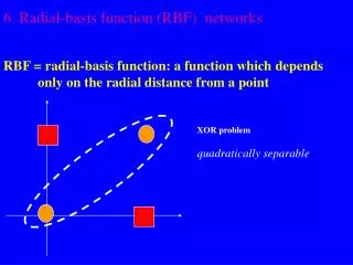
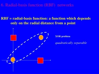
x2 (0,1) (1,1) 0 1 y x1 (0,0) (1,0) Example: the XOR problem • Input space: • Output space: • Construct an RBF pattern classifier such that: (0,0) and (1,1) are mapped to 0, class C1 (1,0) and (0,1) are mapped to 1, class C2 Radial Basis Function Network
φ2 (0,0) Decision boundary 1.0 0.5 (1,1) 1.0 φ1 0.5 (0,1) and (1,0) Example: the XOR problem • In the feature (hidden) space: • When mapped into the feature space < 1 , 2 >, C1 and C2become linearly separable. Soa linear classifier with 1(x) and 2(x) as inputs can be used to solve the XOR problem. Radial Basis Function Network
Learning Algorithms • Parameters to be learnt are: • centers • spreads • weights • Different learning algorithms Radial Basis Function Network
Learning Algorithm 1 • Centers are selected at random • center locations are chosen randomly from the training set • Spreads are chosen by normalization: Radial Basis Function Network
Learning Algorithm 1 • Weights are found by means of pseudo-inverse method Desired response Pseudo-inverse of Radial Basis Function Network
Learning Algorithm 2 • Hybrid Learning Process: • Self-organized learning stage for finding the centers • Spreads chosen by normalization • Supervised learning stage for finding the weights, using LMS algorithm Radial Basis Function Network
Learning Algorithm 2: Centers • K-means clustering algorithm for centers • Initialization: tk(0) random k = 1, …, m1 • Sampling: draw x from input space C • Similaritymatching: find index of best center • Updating: adjust centers • Continuation: increment n by 1, goto 2 and continue until no noticeable changes of centers occur Radial Basis Function Network
Instantaneous error function Learning rate for Depending on the specific function can be computed using the chain rule of calculus Learning Algorithm 3 • Supervised learning of all the parameters using the gradient descent method • Modify centers Radial Basis Function Network
Learning Algorithm 3 • Modify spreads • Modify output weights Radial Basis Function Network
Comparison with multilayer NN RBF-Networks are used to perform complex (non-linear) pattern classification tasks. Comparison between RBFnetworks and multilayer perceptrons: • Both are examples of non-linear layered feed-forward networks. • Both are universal approximators. • Hidden layers: • RBF networks have one single hidden layer. • MLP networks may have more hidden layers. Radial Basis Function Network
Comparison with multilayer NN • Neuron Models: • The computation nodes in the hidden layer of a RBF network are different. They serve a different purpose from those in the output layer. • Typically computation nodes of MLP in a hidden or output layer share a common neuron model. • Linearity: • The hidden layer of RBF is non-linear, the output layer of RBF is linear. • Hidden and output layers of MLP are usually non-linear. Radial Basis Function Network
Comparison with multilayer NN • Activation functions: • The argument of activation function of each hidden unit in a RBF NN computes the Euclidean distance between input vector and the center of that unit. • The argument of the activation function of each hidden unit in a MLP computes the inner product of input vector and the synaptic weight vector of that unit. • Approximations: • RBF NN using Gaussian functions construct local approximations to non-linear I/O mapping. • MLP NN construct global approximations to non-linear I/O mapping. Radial Basis Function Network