Radial Basis-Function Networks

1. Radial Basis-Function Networks

2. Back-Propagation • Stochastic Back-Propagation Algorithm • Step by Step Example • Radial Basis-Function Networks • Gaussian response function • Location of center u • Determining sigma • Why does RBF network work

3. Back-propagation • The algorithm gives a prescription for changing the weights wij in any feed-forward network to learn a training set of input output pairs {xd,td} • We consider a simple two-layer network

4. xk x1 x2 x3 x4 x5

5. Given the pattern xd the hidden unit j receives a net input • and produces the output

6. Output unit i thus receives • And produce the final output

7. In our example E becomes • E[w] is differentiable given f is differentiable • Gradient descent can be applied

8. Consider a network with M layers m=1,2,..,M • Vmi from the output of the ith unit of the mth layer • V0i is a synonym for xi of the ith input • Subscript m layers m’s layers, not patterns • Wmij mean connection from Vjm-1 to Vim

9. Stochastic Back-Propagation Algorithm (mostly used) • Initialize the weights to small random values • Choose a pattern xdk and apply is to the input layer V0k= xdk for all k • Propagate the signal through the network • Compute the deltas for the output layer • Compute the deltas for the preceding layer for m=M,M-1,..2 • Update all connections • Goto 2 and repeat for the next pattern

10. Example w1={w11=0.1,w12=0.1,w13=0.1,w14=0.1,w15=0.1} w2={w11=0.1,w12=0.1,w13=0.1,w14=0.1,w15=0.1} w3={w11=0.1,w12=0.1,w13=0.1,w14=0.1,w15=0.1} W1={w11=0.1,w12=0.1,w13=0.1} W2={w11=0.1,w12=0.1,w13=0.1} X1={1,1,0,0,0}; t1={1,0} X2={0,0,0,1,1}; t1={0,1}

11. net11=1*0.1+1*0.1+0*0.1+0*0.1+0*0.1 V11=f(net11 )=1/(1+exp(-0.2))=0.54983 V12=f(net12 )=1/(1+exp(-0.2))=0.54983 V13=f(net13 )=1/(1+exp(-0.2))=0.54983

12. net11=0.54983*0.1+ 0.54983*0.1+ 0.54983*0.1= 0.16495 o11=f(net11)=1/(1+exp(- 0.16495))= 0.54114 net12=0.54983*0.1+ 0.54983*0.1+ 0.54983*0.1= 0.16495 o12=f(net11)=1/(1+exp(- 0.16495))= 0.54114

13. We will use stochastic gradient descent with =1

14. 1=(1- 0.54114)*(1/(1+exp(- 0.16495)))*(1-(1/(1+exp(- 0.16495))))=0.11394 • 2=(0- 0.54114)*(1/(1+exp(- 0.16495)))*(1-(1/(1+exp(- 0.16495))))= -0.13437

16. 1= 1/(1+exp(- 0.2))*(1- 1/(1+exp(- 0.2)))*(0.1* 0.11394+0.1*( -0.13437)) 1=-5.0568e-04 2=-5.0568e-04 3=-5.0568e-04

17. First Adaptation for x1(one epoch, adaptation over all training patterns, in our case x1x2) 1=-5.0568e-04 1=0.11394 2=-5.0568e-04 2= -0.13437 3=-5.0568e-04 x1 =1 v1=0.54983 x2 =1 v2=0.54983 x3 =0 v3=0.54983 x4 =0 x5 =0

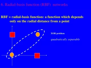
18. Radial Basis-Function Networks • RBF networks train rapidly • No local minima problems • No oscillation • Universal approximators • Can approximate any continuous function • Share this property with feed forward networks with hidden layer of nonlinear neurons (units) • Disadvantage • After training they are generally slower to use

20. Gaussian response function • Each hidden layer unit computes • x = an input vector • u = weight vector of hidden layer neuron i

21. The output neuron produces the linear weighted sum • The weights have to be adopted • (LMS)

22. The operation of the hidden layer • One dimensional input

23. Two dimensional input

24. Every hidden neuron has a receptive field defined by the basis-function • x=u, maximum output • Output for other values drops as x deviates from u • Output has a significant response to the input x only over a range of values of x called receptive field • The size of the receptive field is defined by • umay be called mean and  standard deviation • The function is radially symmetric around the mean u

25. Location of centers u • The location of the receptive field is critical • Apply clustering to the training set • each determined cluster center would correspond to a center u of a receptive field of a hidden neuron

26. Determining  • The object is to cover the input space with receptive fields as uniformly as possible • If the spacing between centers is not uniform, it may be necessary for each hidden layer neuron to have its own  • For hidden layer neurons whose centers are widely separated from others,  must be large enough to cover the gap

27. Following heuristic will perform well in practice • For each hidden layer neuron, find the RMS distance between ui and the center of its N nearest neighbors cj • Assign this value to i

30. f( ) f( ) f( ) f( ) f( ) f( ) f( ) f( ) f( ) f( ) f( ) f( ) f( ) f( ) f( ) f( ) Why does a RBF network work? • The hidden layer applies a nonlinear transformation from the input space to the hidden space • In the hidden space a linear discrimination can be performed

32. Back-Propagation • Stochastic Back-Propagation Algorithm • Step by Step Example • Radial Basis-Function Networks • Gaussian response function • Location of center u • Determining sigma • Why does RBF network work

33. Bibliography • Wasserman, P. D., Advanced Methods in Neural Computing, New York: Van Nostrand Reinhold, 1993 • Simon Haykin, Neural Networks, Secend edition Prentice Hall, 1999

34. Support Vector Machines