Download

1 / 38
390 likes | 643 Views
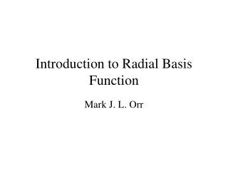
Radial-Basis Function Networks. CS/CMPE 537 – Neural Networks. Introduction. Typical tasks performed by neural networks are association, classification, and filtering. This categorization has historical significance as well.

E N D
Radial-Basis Function Networks CS/CMPE 537 – Neural Networks
Introduction • Typical tasks performed by neural networks are association, classification, and filtering. This categorization has historical significance as well. • These tasks involve input-output mappings, and the network is designed to learn the mapping from knowledge of the problem environment • Thus, the design of a neural network can be viewed as a curve-fitting or function approximation problem • This viewpoint is the motivation for radial-basis function networks CS/CMPE 537 - Neural Networks (Sp 2006-2007) - Asim Karim @ LUMS
Radial-Basis Function Networks • RBF are 2 layer networks; input source nodes, hidden neurons with basis functions (nonlinear), and output neurons with linear/nonlinear activation functions • The theory of radial-basis function networks is built upon function approximation theory in mathematics • RBF networks were first used in 1988. Major work was done by Moody and Darken (1989) and Poggio and Girosi (1990) • In RBF networks, the mapping from input to high-dimension hidden space is nonlinear, while that from hidden to output space is linear • What is the basis for this ? CS/CMPE 537 - Neural Networks (Sp 2006-2007) - Asim Karim @ LUMS
Radial-Basis Function Network Φ1(.) w x1 y1 y2 xp ΦM(.) Source nodes Hidden neurons with RBF activation functions Output neurons CS/CMPE 537 - Neural Networks (Sp 2006-2007) - Asim Karim @ LUMS
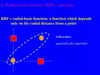
Cover’s Theorem (1) • Cover’s theorem (1965) gives the motivation for RBF networks • Cover’s theorem on the separability of patterns • Complex pattern-classification problems cast in high-dimensional space nonlinearly is more likely to be linearly separable than low-dimensional space CS/CMPE 537 - Neural Networks (Sp 2006-2007) - Asim Karim @ LUMS
Cover’s Theorem (2) • Consider set X of N p-dimensional vectors (input patterns) x1 to xN. Let X+ and X- be a binary partition of X, and φ(x) = [φ1(x), φ2(x),…, φM(x)]T. • Cover’s theorem • A binary partition (dichotomy) [X+, X-] of X is said to be φ-separable if there exist an m-dimensional vector w such that wTφ(x) ≥ 0 when x belong to X+ wTφ(x) < 0 when x belong to X- • Decision boundary or surface wTφ(x) = 0 CS/CMPE 537 - Neural Networks (Sp 2006-2007) - Asim Karim @ LUMS
Cover’s Theorem (3) CS/CMPE 537 - Neural Networks (Sp 2006-2007) - Asim Karim @ LUMS
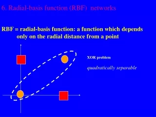
Example (1) • Consider the XOR problem to illustrate the significance of φ-separability and Cover’s theorem. • Define a pair of Gaussian hidden functions φ1(x) = exp(-||x – t1||2) t1 = [1, 1]T φ2(x) = exp(-||x – t2|2|) t1 = [0, 0]T • Output of these function for each pattern CS/CMPE 537 - Neural Networks (Sp 2006-2007) - Asim Karim @ LUMS
Example (2) CS/CMPE 537 - Neural Networks (Sp 2006-2007) - Asim Karim @ LUMS
Function Approximation (1) • Function approximation seeks to describe the behavior of complex functions by ensembles of simpler functions • Describe f(x) by F(x) • F(x) can be described in a compact region of input space by F(x) = Σi=1N wiφi(x) Such that |f(x) – F(x)| < ε • ε can be made arbitrarily small • Choice of function φ(.) ? CS/CMPE 537 - Neural Networks (Sp 2006-2007) - Asim Karim @ LUMS
Function Approximation (2) • Find F(x) that “best” approximates the map/function f. The best approximation is problem dependent, and it can be strict interpolation or good generalization (regularized interpolation). • Design decisions • Choice of elementary functions φ(.) • How to compute the weights w ? • How many elementary functions to use (i.e. what should be N)? • How to obtain a good generalization ? CS/CMPE 537 - Neural Networks (Sp 2006-2007) - Asim Karim @ LUMS
Choice of Elementary Functions φ • Let f(x) belongs to the function space L2(Rp) (true for almost all physical systems) • We want φ to be a basis of L2 • What is meant by a basis? • A set of functions φi (i = 1, M) are a basis of L2 if linear superposition of φi can generate any function in L2 . Moreover, they must be linearly independent: w1φ1 + w2φ2 +…+ wMφM = 0 iff wi = 0 for all i CS/CMPE 537 - Neural Networks (Sp 2006-2007) - Asim Karim @ LUMS
Interpolation Problem (1) • In general, the map from an input space to an output space is given by f: Rp -> Rq • p and q = input and out space dimensions; f = map or hypersurface • Strict interpolation problem • Given a set of N different points xi (i = 1, N) and a corresponding set of N real numbers di (i = 1, N) find a function F: Rp -> R1 that satisfies the interpolation condition F(xi) = di i = 1, N • The function F passes through all the points CS/CMPE 537 - Neural Networks (Sp 2006-2007) - Asim Karim @ LUMS
Interpolation Problem (2) • A common type of φ(.) is radial-symmetric basis functions F(x) = Σi=1N wiφ||x – xi|| Substituting and writing in matrix format Фw = d • Ф = φji (i, j = 1, N) = interpolation matrix; φji = φ||xj – xi|| • w = linear weight vector; d = desired response vector CS/CMPE 537 - Neural Networks (Sp 2006-2007) - Asim Karim @ LUMS
Interpolation Problem (3) • Ф is known to be positive definite for a certain class of radial-basis functions. Thus, w = Ф-1d • In theory, w can be computed. In practice, however, Ф is close to singular • Then what ? • Regularization theory to perturb Ф to make it non-singular • But, there is another problem… poor generalization or overfitting CS/CMPE 537 - Neural Networks (Sp 2006-2007) - Asim Karim @ LUMS
Ill-Posed Problems • Supervised learning is a an ill-posed problem • There is not enough information in the training data to reconstruct the input-output mapping uniquely • The presence of noise or imprecision in the input data adds uncertainty to the reconstruction of the input-outut mapping • To achieve good generalization additional information of the domain is needed • In other words, the input-output patterns should exhibit redundancy • Redundancy is achieved when the physical generator of data is smooth, and thus can be used to generate redundant input-output examples CS/CMPE 537 - Neural Networks (Sp 2006-2007) - Asim Karim @ LUMS
Regularization Theory (1) • How to make an ill-posed problem well-posed ? • By constraining the mapping with additional information (e.g. smoothness) in the form of a nonnegative functional • Proposed by Tikhonov in 1963 in the context of function approximation in mathematics CS/CMPE 537 - Neural Networks (Sp 2006-2007) - Asim Karim @ LUMS
Regularization Theory (2) • Input-output examples: xi, di (i = 1, N) • Find the mapping F(x): Rp -> R1 for the input-output examples • In regularization theory, F is found by minimizing the cost functional ξ(F) ξ(F) = ξs(F) + λξc(F) • Standard error term ξs(F) = 0.5Σi=1N (di – yi)2 = 0.5Σi=1N (di – F(xi))2 • Regularization term ξc(F) = 0.5||PF(x)||2 • P = linear differential operator CS/CMPE 537 - Neural Networks (Sp 2006-2007) - Asim Karim @ LUMS
Regularization Theory (3) • Regularization term depends on the geometric properties of the approximating function • The selection of the operator P is therefore problem dependent based on prior knowledge of the geometric properties of the actual function f(x) (e.g. the smoothness of f(x)) • Regularization parameter λ: a positive real number • This parameter indicates the sufficiency of the given input-output examples in capturing the underlying function f(x) • The solution of the regularization problem is a function type F(x) • We won’t go into the details of how to find F as it requires good understanding of functional analysis CS/CMPE 537 - Neural Networks (Sp 2006-2007) - Asim Karim @ LUMS
Regularization Theory (4) • Solution of the regularization problem yields F(x) = 1/λΣi=1N [di - F(xi)]G(x, xi) = Σi=1N wiG(x, xi) • G(x,xi) = Green’s function centered on xi • In matrix form F = Gw or (G + λI)w = d and w = (G + λI)-1d • G depends only on the operator P CS/CMPE 537 - Neural Networks (Sp 2006-2007) - Asim Karim @ LUMS
Type of Function G(x; xi) • If P is translationally invariant then G(x; xi) depends only on the difference of x and xi, i.e. G(x; xi) = G(x - xi) • If P is both translationally and rotationally invariant then G(x; xi) depends only on Euclidean norm of the difference vector x - xi, i.e. G(x; xi) = G(||x – xi||) • This is a radial-basis function • If P is further constrained, and G(x; xi) is positive definite, then we have the Gaussian radial-basis function, i.e. G(x; xi) = exp(- (1/2σ2) ||x – xi||2) CS/CMPE 537 - Neural Networks (Sp 2006-2007) - Asim Karim @ LUMS
Regularization Network (1) CS/CMPE 537 - Neural Networks (Sp 2006-2007) - Asim Karim @ LUMS
Regularization Network (2) • The regularization network is based on the regularized interpolation problem F(x) = Σi=1N wiG(x, xi) • It has 3 layers • Input layer of p source nodes, where p is the dimension of the input vector x (or number of independent variables) • Hidden layer with N neurons, where N is the number of input-output examples. Each neuron uses the activation function G(x; xi) • Output layer with q neurons, where q is the output dimension • The unknowns are the weights w (only) from the hidden layer to the output layer CS/CMPE 537 - Neural Networks (Sp 2006-2007) - Asim Karim @ LUMS
RBF Networks (in Practice) (1) • The regularization network requires N hidden neurons, which becomes computationally expensive for large N • The complexity of the network is reduced to obtain an approximate solution to the regularization problem • The approximate solution F*(x) is then given by F*(x) = Σi=1M wiφi(x) • φi(x) (i = 1,M) = new set of basis functions; M is typically less than N • Using radial basis functions F*(x) = Σi=1M wiφi(||x – ti||) CS/CMPE 537 - Neural Networks (Sp 2006-2007) - Asim Karim @ LUMS
RBF Networks (2) CS/CMPE 537 - Neural Networks (Sp 2006-2007) - Asim Karim @ LUMS
RBF Networks (3) • Unknowns in the RBF network • M, the number of hidden neurons (M < N) • The centers ti of the radial-basis functions • And the weights w CS/CMPE 537 - Neural Networks (Sp 2006-2007) - Asim Karim @ LUMS
How to Train RBF Networks - Learning • Normally the training of the hidden layer parameters (number of hidden neurons, centers and variance of Gaussian) is done prior to the training of the weights (i.e. on a different ‘time scale’) • This is justified based on the fact that the hidden layer performs a different task (nonlinear) than the output layer weights (linear) • The weights are learned by supervised learning using an appropriate algorithm (LMS or BP) • The hidden layer parameters are learned by (in general, but not always) unsupervised learning CS/CMPE 537 - Neural Networks (Sp 2006-2007) - Asim Karim @ LUMS
Fixed Centers Selected at Random • Randomly select M inputs as centers for the activation functions • Fix the variance of the Gaussian based on the distance between the selected centers. A radial-basis function centered at ti is then given by φ(||x – ti||) = exp(- M/d2 ||x – ti||2) • d = max. distance between the chosen centers • The width’ or standard deviation of the functions is fixed, given by σ = d/√2M • The linear weights are then computed by solving the regularization problem or by using supervised learning CS/CMPE 537 - Neural Networks (Sp 2006-2007) - Asim Karim @ LUMS
Self-Organized Selection of Centers • Use a self-organizing or clustering technique to determine the number and centers of the Gaussian functions • A common algorithm is the k-means algorithm. This algorithms assigns a label to a vector x by the majority label on the k-nearest neighbors • Then compute the weights using a supervised error-correction learning such as LMS CS/CMPE 537 - Neural Networks (Sp 2006-2007) - Asim Karim @ LUMS
Supervised Selection of Centers • All unknown parameters are trained using error-correcting supervised learning • A gradient descent approach is used to find the minimum of the cost function wrt the weights wi and activation function centers ti and spread of centers σ CS/CMPE 537 - Neural Networks (Sp 2006-2007) - Asim Karim @ LUMS
Example (1) • Classify between two ‘overlapping’ two-dimensional, Gaussian-distributed patterns • Conditional probability density function for the two classes f(x | C1) = 1/2πσ12 exp[-1/2σ12 ||x – μ1||2] μ1 = mean = [0 0]T and σ12 = variance = 1 f(x | C2) = 1/2πσ22 exp[-1/2σ22 ||x – μ2||2] μ2 = mean = [2 0]T and σ22 = variance = 4 • x = [x1 x2]T = two dimensional input • C1 and C2 = class labels CS/CMPE 537 - Neural Networks (Sp 2006-2007) - Asim Karim @ LUMS
Example (2) CS/CMPE 537 - Neural Networks (Sp 2006-2007) - Asim Karim @ LUMS
Example (3) CS/CMPE 537 - Neural Networks (Sp 2006-2007) - Asim Karim @ LUMS
Example (4) • Consider a two-input, M hidden neurons, and two-output RBF • Decision rule: an input x is classified to C1 if y1 >= 0 • The training set is generated from the probability distribution functions • Using the perceptron algorithm, the network is trained for minimum mean-square-error • The testing set is generated from the probability distribution functions • The trained network is tested for correct classification • For other implementation details, see the Matlab code CS/CMPE 537 - Neural Networks (Sp 2006-2007) - Asim Karim @ LUMS
Example: Function Approximation (1) • Approximate relationship between a car’s fuel economy (in miles per gallon) and its characteristics • Input data description: 9 independent discrete valued, boolean, and continuous variables • X1: number of cylinders • X2: displacement • X3: horsepower • X4: weight • X5: acceleration • X6: model year • X7: Made in US? (0,1) • X8: Made in Europe? (0,1) • X9: Made in Japan? (0,1) • Output f(X) is fuel economy in miles per gallon CS/CMPE 537 - Neural Networks (Sp 2006-2007) - Asim Karim @ LUMS
Example: Function Approximation (2) • Using the NNET toolbox, create and train a RBF network with function newrb • The function parameters allows you to set the mean-squared-error goal of the training, the spread of the radial-basis functions, and the maximum number of hidden layer neurons. • Newrb uses the following approach to find the unknowns (it is a self-organizing approach) • Start with one hidden neuron; compute network error • Add another neuron with center equal to input vector that produced the maximum error; compute network error • If network error does not improve significantly, stop; other go to previous step and add another neuron CS/CMPE 537 - Neural Networks (Sp 2006-2007) - Asim Karim @ LUMS
Comparison of RBF Network and MLP (1) • Both are universal approximators. Thus, a RBF network exists for every MLP, and vice versa • An RBF has a single hidden layer, while an MLP can have multiple hidden layers • The model of the computational neurons of an MLP are all identical, while the neurons in the hidden and output layers of an RBF network have different models • The activation functions of the hidden nodes of an RBF network is based on the Euclidean norm of the input wrt to a center, while that of an MLP is based on the inner product of input and weights CS/CMPE 537 - Neural Networks (Sp 2006-2007) - Asim Karim @ LUMS
Comparison of RBF Network and MLP (2) • MLPs construct global approximations to nonlinear input-output mapping. This is a consequence of the global activation function (sigmoidal) used in MLPs • As a result, MLP can perform generalization in regions where input data is not available (i.e. extrapolation) • RBF networks construct local approximations to input-output data. This is a consequence of the local Gaussian functions • As a result, RBF networks are capable of fast learning from the training data CS/CMPE 537 - Neural Networks (Sp 2006-2007) - Asim Karim @ LUMS