Download
1 / 61
650 likes | 1.13k Views
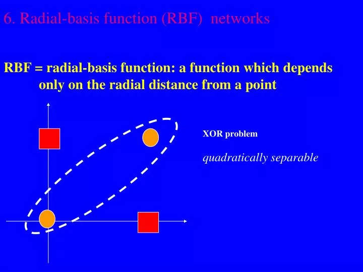
6. Radial-basis function (RBF) networks RBF = radial-basis function : a function which depend s only on the radial distance from a point. XOR problem quadratically separable . So RBFs are functions taking the form

E N D
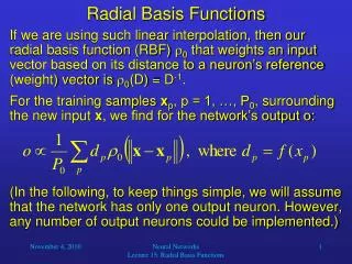
6. Radial-basis function (RBF) networks RBF = radial-basis function: a function which depends only on the radial distance from a point XOR problem quadratically separable
So RBFs are functions taking the form Where f is a nonlinear activation function, xis the input and xi is the i’th position, prototype, basis orcentrevector. The idea is that points near the centres will have similar outputs I.e. if x ~ xi then f(x) ~f(xi) since they should have similar properties. Therefore instead of looking at the data points themselves characterise the data by their distances from the prototype vectors (similar to kernel density estimation)
For example, the simplest form of fis the identity function f(x) = x x1=(0,1) x d1 d2 (0,0) 1 1.1 (1,1) 1 .5 (0,1) 0 1.1 (1,0) .5 x2=(1,0.5) Now use the distances as the inputs to a network and form a weighted sum of these
Can be viewed as a Two-layer network y1 y2 Input Output d wj yM fN (y)=f |y-xN| Hidden layer output = S wifi(y) adjustable parameters are weights wj number of hidden units = number of prototype vectors Form of the basis functions decided in advance
use a weighted sum of the outputs from the basis functions for e.g. classification, density estimation etc • Theory can be motivated by many things (regularisation, Bayesian classification, kernel density estimation, noisy interpolation etc), but all suggest that basis functions are set so as to represent the data. • Thus centres can be thought of as prototypes of input data. * * * * 1 0 * * 0 O1 MLP vs RBF distributed local
E.g. Bayesian interpretation: if we choose to model the probability and we choose appropriate weights then we can interpret the outputs as the posterior probabilities: Ok = P(Ck|(x) a p(x|Ck) P(Ck) O1 O2 O3 0 0 P(C1) P(C3) F1(x) = p(x|C1) F3(x) = p(x|C3) x y
Starting point: exact interpolation Each input pattern x must be mapped onto a targetvalue d d x
That is, given a set of N vectorsxi and a corresponding set of N real numbers, di (the targets), find a function F that satisfies the interpolation condition: F ( xi ) = di fori =1,...,N or more exactly find: satisfying:
Example: XOR problem x d (0,0) 0 (1,1) 0 (0,1) 1 (1,0) 1 Exact interpolation: RBF placed at position of each pattern vector using 1) linear RBF
w i.e. 4 hidden units in network Network structure
w1 w2 w3 w4 0 1 1 1 0 1 1 0 1 1 1 0 0 1 1 0 = w1 w2 w3 w4 1 1 Results =
And general solution is: Ie F(x1,x2) = sqrt(x12+x22) sqrt((x1-1)2+x22) sqrt(x12+(x2-1)2) + sqrt((x1-1)2+(x2-1)2)
For n vectors get: f ( x1- x1 ) w1 wN d1 dN f ( x1 - xN) = f ( xN - xN ) f ( xN - x1) Interpolation Matrix weight f ( xi - xj ): scalarfunction of distance between vector xi and xj Equivalently FW = D
If F is invertible we have a unique solution of the above equation Micchelli’s Theorem Let xi , i = 1, ..., N be a set of distinct points in Rd, Then the N-by-N interpolation matrix , whose ji-th element is f ( xi - xj ) , is nonsingular. So provided F is nonsingular then interpolation matrix will have an inverse and weights to achieve exact interpolation
Easy to see that there is always a solution. For instance, if we take f(x-y)=1 if x= y, and 0 otherwise (e.g. a Gaussian with very small s), setting wi=disolves the interpolation problem However, this is a bit trivial as the only general conclusion about the input space is that the training data points are different.
To summarize: • For a given data set containing N points (xi,di), i=1,…,N • Choose a RBF function f • Calculate f(xj - xi ) • Obtain the matrixF • Solve the linear equationFW = D • Get the unique solution • Done! Like MLP’s, RBFNs can be shown to be able to approximate any function to arbitrary accuracy (using an arbitrarily large numbers of basis functions). Unlike MLP’s, however, they have the property of ‘best approximation’ i.e. that there exists an RBFN with minimum approximation error.
Other types of RBFs include • Multiquadrics • for some c>0 • (b) Inverse multiquadrics • for some c>0 • Gaussian • for some s >0
Linear activation function has some undesirable properties e.g. f(xi) = 0. (NBfis still a non-linear function as it is only piecewise linear in x). • Inverse multiquadrics and Gaussian RBFs are both examples • of ‘localized’ functions • Multiquadrics RBFs are ‘nonlocalized’ functions
‘Localized’: as distance from the centre increasesthe output of the RBF decreases
‘Nonlocalized’: as distance from the centre increasesthe output of the RBF increases
Example: XOR problem x d (0,0) 0 (1,1) 0 (0,1) 1 (1,0) 1 Exact interpolation: RBF placed at position of each pattern vector using 2) Gaussian RBF with s=1
w i.e. 4 hidden units in network Network structure
w1 w2 w3 w4 exp(0) exp(-.5) exp(-.5) exp(-1) exp(-.5) exp(0) exp(-1) exp(-.5) exp(-.5) exp(-1) exp(0) exp(-.5) exp(-1) exp(-.5) exp(-.5) exp(0) 0 1 1 0 = w1 w2 w3 w4 -3.0359 3.4233 3.4233 -3.0359 Results =
1) f(x1,x2) = sqrt(x12+x22) - sqrt((x1-1)2+x22) - sqrt(x12+(x2-1)2) + sqrt((x1-1)2+(x2-1)2) 2) f(x1,x2) = -3.0359 exp(-(x12+x22)/2) +3.4233 exp(-(x1-1)2+x22)/2) +3.4233 exp(-(x12+(x2-1)2)/2) -3.0359 exp(-(x1-1)2+(x2-1)2)/2)
Problems with exact interpolation can produce poor generalisation performance as only data points constrain mapping overfitting problem Bishop(1995) example Underlying function f(x)=0.5+0.4sine(2pi x) sampled randomly for 30 points added gaussian noise to each data point 30 data points 30 hidden RBF units fits all data points but creates oscillations due added noise and unconstrained between data points
All Data Points 5 Basis functions
To fit an rbf to every data point is very inefficient due to the computational cost of matrix inversion and is very bad for generalisation so: • Use less RBF’s than data pointsI.e. M<N • Therefore don’t necessarily have RBFs centred at data points • Can include bias terms • Can have gaussians with general covariance matrices but there is a trade-off between complexity and the number of parameters to be found
1 parameter d parameters for d rbfs we have d(d+1)/2 parameters
6. Radial-basis function (RBF) networks II Generalised radial basis function networks Exact interpolation expensive due to cost of matrix inversion prefer fewer centres (hidden RBF units) centres not necessarily at data points can include biases can have general covariance matrices now no longer exact interpolation, so where M (number of hidden units) <N (number of training data)
Three-layer networks f0= 1 x1 x2 w0 = bias Input: nD vector Output y wM fM(x)=f (x-xM) xN Hidden layer • output = S wifi(x) • adjustable parameters are weights wj, number of hidden units M (<N) • Form of the basis functions decided in advance
F(x) F(x) S S w1 w2 w31 w32 sig(w1Tx) f(r1) f(r2) sig(w2Tx) * w1 w2 r2 * x x r1 w1Tx = k
Comparison of MLP to RBFN MLP hidden unit outputs are monotonic functions of a weighted linear sum of the inputs => constant on (d-1)D hyperplanes distributed representation as many hidden units contribute to network output => interference between units => non-linear training => slow convergence RBF hidden unit outputs are functions of distance from prototype vector (centre) => constant on concentric (d-1)D hyperellipsoids localised hidden units mean that few contribute to output => lack of interference => faster convergence
Comparison of MLP to RBFN MLP more than one hidden layer global supervised learning of all weights global approximations to nonlinear mappings RBF one hidden layer hybrid learning with supervised learning in one set of weights localised approximations to nonlinear mappings
Three-layer networks f0= 1 x1 x2 w0 = bias Input: nD vector Output y wM fM(x)=f (x-xM) xN Hidden layer • output = S wifi(x) • adjustable parameters are weights wj, number of hidden units M (<N) • Form of the basis functions decided in advance
Hybrid training of RBFN Two stage ‘hybrid’ learning process stage 1: parameterise hidden layer of RBFs - hidden unit number (M) -centre/position (ti) -width (s) use unsupervised methods (see below) as they are quick and unlabelled data is plentiful. Idea is to estimate the density of the data stage 2 Find weight values between hidden and output units minimize sum-of-squares error between actual output and desired responses --invert matrix F if M=N --Pseudoinverse of F if M<N Stage 2 later, now concentrate on stage 1.
Random subset approach Randomly select centres of M RBF hidden units from N data points widths of RBFs usually common and fixed to ensure a degree of overlap but based on an average or maximum distance between RBFs e.g. s = dmax /sqrt (2M) where dmax is the maximum distance between the set of M RBF units The method is efficient and fast, but suboptimal and its important to get s correct …
s =10 s =0.08 s =0.4
Clustering Methods: K-means algorithm --divides data points into K subgroups based on similarity Batch version 1. Randomly assign each pattern vector x to one of K subsets 2. Compute mean vector of each subset 3. Reassign each point to subset with closest mean vector 4. Until no further reassignments, loop back to 2 On-line version 1. Randomly choose K data points to be basis centres mi 2. As each vector is xn presented, update the nearest mi using: Δmi = h(xn - mi) 3. Repeat until no further changes
The covariance matrices (s) can now be set to the covariance of the data points of each subset -- However, note that K must be decided at the start -- Also, the algorithm can be sensitive to initial conditions -- Can get problems of no/few points being in a set: see competitive learning lecture -- Might not cover the space accurately Other unsupervised techniques such as self organising maps and Gaussian mixture models can also be used Another approach is to use supervised techniques where the parameters of the basis functions are adaptive and can be optimised. However, this negates the speed and simplicity advantages of the 1st stage of training.
y * * X * x h * * * Relationship with probability density function estimation Radial basis functions can be related to kernel density functions (Parzen windows) used to estimate probability density functions E.g. In 2 dimensions the pdf at a point x can be estimated from the fraction of training points which fall within a square of side h centred on x Here p(x) = 1/6 x 1/(hxh) xSn H(x-xn,h) where H = 1 if |xn-x| < h ie estimate density by fraction of points within each square Alternatively, H(|xn-x|) could be gaussian giving a smoother estimate for the pdf
In Radial basis networks the first stage of training is an attempt to model the density of the data in an unsupervised way As in kernel density estimation, we try to get an idea of the underlying density by picking some prototypical points Then use distribution of the data to approximate a prior distribution
Back to Stage 2 for a network with M < N basis vectors Now for each training data vector ti and corresponding target di we want F ( ti ) = di , that is, we must find a function F that satisfies the interpolation condition: F ( ti ) = di fori =1,...,N Or more exactly find: satisfying:
1 f ( t1- x1 ) w0 w1 wM d1 dN f ( t1 - xM) = f ( tN - xN ) 1 f ( tN - x1) So the interpolation matrix becomes: Which can be written as: FW = D where Fis an MxN matrix (not square).
To solve this we need to generate an error function such as the least squares error: and minimise it. As the derivative of the least squares error is a linear function of the weights it can be solved using linear matrix inversion techniques (usually singular value decomposition (Press et al., Numerical Recipes)). Other error functions can be used but minimising the error then becomes a non-linear optimisation problem.
However, note that the problem is OverDetermined That is, by using N training vectors and only M centres we have M unknowns (the weights) and N bits of information eg training vectors (-2, 0), (1, 0), targets 1, 2 centre: (0, 0), linear rbf FW = D => w =0.5 or w =2 ??? Unless N=M and there are no degeneracies (parallel or nearly parallel) data vectors, we cannot simply invert the matrix and must use the pseudoinverse (using Singular Value Decomposition).
Alternatively, can view this as an ill-posed problem Ill-posed problems (Tikhonov) How do we infer function F which maps X onto y from a finite data set? This can be done if problem is well-posed - existence = each input pattern has an output - uniqueness = each input pattern maps onto only one output - continuity = small changes in input pattern space imply small changes in y In RBFs however: - noise can violate continuity condition - different output values for same input patterns violates uniqueness - insufficient information in training data may violate existence condition
Ill-posed problem: the finite data set does not yield a unique solution
Regularization theory (Tikhonov, 1963) • To solve ill-posed problems need to supplement finite data set • with prior knowledge about nature of mapping • -- regularization theory • common to place constraint that mapping is smooth (since smoothness implies continuity) • add penalty term to standard sum-of squares error for non-smooth mappings • E(F)=ES (F)+ l Ec(F) • where eg: • ES (F)= 1/2 S ( di- F(xi) )2 and Ec(F)=1/2 || DF ||2 • and DF could be, say the first or second order derivative of F etc.