Download
1 / 48
480 likes | 600 Views
Numerical weather prediction from short to long range Predicting uncertainty. Pierre Eckert Head of regional office, MeteoSwiss, Geneva. Topics. Global models (ECMWF) Grids Parameters Data and initialisation Time evolution Products Regional models (COSMO)

E N D
Numerical weather prediction from short to long rangePredicting uncertainty Pierre Eckert Head of regional office, MeteoSwiss, Geneva
Topics • Global models (ECMWF) • Grids • Parameters • Data and initialisation • Time evolution • Products • Regional models (COSMO) • Chaos and ensemble forecasting (EPS) • Probabilistic forecasts • Monthly and seasonal forecasting • Climate models
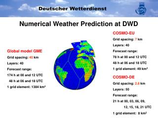
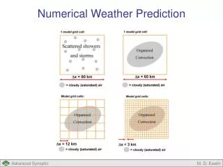
Global model: horizontal grid Latitude-longitude gridding of the planet. Present resolution at ECMWF: about 25 km (ECMWF = European Centre for Medium range Weather Forecast) About 800’000 grid points
Vertical levels Vertical levels follow the orography 91 levels in the ECMWF model 800’000 x 91 = 75’000’000 coordinate points
Meteorological parameters • Température • Wind (2 horizontal dimensions) • Humidity (quantity of water vapour) • Quantity of liquid water • Quantity of ice Pressure and vertical wind are deduced (from temperature and horizontal wind) • 6 variables on each of the 75’000’000 points • The state of the atmosphere is described by about 450 millions of numbers.
Analysis • The analysis procedure aims to determine all parameters of the model at a time t (for example 00z et 12z). • Most of the available observations is used. • These observations do not usually lie on the coordinate points of the model, nor at the eact analysis time. • The analysis process is complex. • The equilibrium of the model has to be kept • « Incoherent » observations have to be rejected • A lot of computing time is already used in this phase
Observations from the ground
Observations of the sea
Geostationary satellites
Polar satellites
Time evolution of the model • Once the initial state is known, the future evolution is computed. • The set of equations from the atmosphere physics is applied (dynamics, thermodynamics) • These equations allow to compute a new state of the model by steps of 10 minutes up to 10 days (240h) • The equations are highly non-linear: the solutions are chaotic (see later)
Example of equation:change of temperature + heat from compression - heat from expansion + head from condensation - heat from evaporation + solar radiation + …
Other global models • GFS (NCEP, USA) • UM, Unified Model (UKMO, UK) • Arpège (MétéoFrance, France) • GME (DWD, Allemagne) • Japan • Korea • …
Regional models • For the moment it is not possible to build models covering the whole planet with resolutions below 10 km (but we are not far!) • Regional models are built in consequence in order to catch regional details in the short range (1-3). • Several consortia or academic initiatives: COSMO, Aladin, HIRLAM, MM5, WRF,… • It is possible to add very local information to the initial state: rainfall rates from radars, wind profilers,…
IFS (ECMWF) COSMO-7 COSMO-2 Radar Model embedding COSMO-7 • 393x338 grid points • 6.6km, 60 levels • 3x72h forecasts per day COSMO-2 • 520x350 grid points • 2.2km, 60 levels • 8x 24h forecasts per day
An approach to chaos • The atmosphere is chaotic: this means: • 1) there is an « attractor » of possible states. This is the climate. • 2) the time evolution is very dependent on the initial conditions (butterfly effect). • Toy model: the Lorenz attractor Weak dependency Strong dependency
An approach to chaos:Ensemble forecasting • Ensemble forecasting (EPS: Ensemble Prediction System) aims at catching the dependency of the weather evolution from the initial state by generating small perturbation of this initial state (50 at ECMWF). • The 50 models have a coarser resolution (~50 km)
Monthly and seasonal forecasts • The model can be integrated for several weeks or months. • The goal is not to produce a forecast for day 25 or week 12. • But it is in principle possible to produce a mean forecast for the week 3 or the month 4. • The ocean temperature cannot be kept constant during this long time. • In addition to the atmospheric model, a model of the ocean has to be built. Variables: speed, temperature, salinity. • This kind of forecast presents good results in the tropics, fair results in north America, poor results over central Europe. • The monthly forecast is run once a week, the seasonal forecast once a month.
Monthly forecast: skill Prévision mensuelle:Températures
Seasonal forecast: skil in summer Temperature
Climate models • Climate models are basically similar to seasonal models • They include a model of the ocean • The difference is that some properties of the atmosphere or boundary conditions can be changed: • Solar irradiation • Aerosols, volcanic ashes • Greenhouse gases: CO2, methane,… • The new equilibrium is computed
Atmospheric radiation balance Absorption bythe atmosphere
Natural and anthropogenic forcing Natural forcing only +1.0 +1.0 +0.5 +0.5 0.0 0.0 Anomaly in °C Anomaly in °C -0.5 -0.5 -1.0 -1.0 1900 1900 1920 1920 1940 1940 1960 1960 1980 1980 2000 2000 Model simulations of the past climate (IPCC 2001, confirmed by IPCC 2007) Observed temperature Observed temperature Range of model simulations Range of model simulations Mean of model simulations Mean of model simulations Source: IPCC 2007; Max Planck Institut Hamburg, 2007
°C A1Fl 6.0 A2 A1B B1 5.0 Constant greenhouse gases concentration 20est century B2 4.0 1250 ppm 3.0 Changes in global surface temperature 850 ppm 2.0 A1T 600 ppm 1.0 0.0 -1.0 1900 2000 2100 Year Projected change of the global temperature until 2100 (IPCC 2007) Concentration of greenhouse gases in CO2-equivalent: B1: 600 ppm A1T: 700 ppm B2: 800 ppm A1B: 850 ppm A2: 1250 ppm A1Fl: 1550 ppm Best estimate: +1.8 ° to +4.0° C
Conclusions • Numerical weather models are able • to use a lot of measurements • to produce useful forecasts in the medium range (up to ~6 days) • to reproduce structures down to the kilometre scale • They have to be interpreted by professional meteorologists • They are able to reproduce the past climate… • … and to estimate the future climate
Discussion How to address climate issues during weather presentations? • How “normal” is the weather today, tomorrow? • Is this storm exceptional • Explain that the fact that a cold January is not incompatible with long term warming. • Give advice on reducing use of fossil fuels (heating, traffic,…)