Download

1 / 43
440 likes | 622 Views
Microarray Normalization. Issues in High-Throughput Data Analysis BIOS 691-803 Spring 2010 Dr Mark Reimers. Normalization of Expression Arrays. Historical approaches 1995-2005 Current standard approaches Q.75 for Agilent Quantile for Affymetrix and Nimblegen VSN for Illumina

E N D
Microarray Normalization Issues in High-Throughput Data Analysis BIOS 691-803 Spring 2010 Dr Mark Reimers
Normalization of Expression Arrays • Historical approaches 1995-2005 • Current standard approaches • Q.75 for Agilent • Quantile for Affymetrix and Nimblegen • VSN for Illumina • Modeling correlation (later) • Technical variable regression (later)
Historic Normalization Approaches • One Parameter • Single reference standard • Total or median brightness • Two parameter or non-parametric • Invariant Set • Lowess for two-color arrays • Matching variance • Distribution matching • By variance or by quantiles • Local approaches • Print-tip separate normalization
Median Normalization • Subtract chip medians from values to align centers of chip intensity distributions
Non-normalized data {(M,A)}n=1..5184: M = log2(R/G) Saturation occurs at different densities for Cy-3 (green) and Cy-5 (red) dyes because different densities of label get attached to the same amount of cDNA target. Model bias by an intensity dependent function c(A) Two-color Intensity-Dependent Bias c(A)
Global normalized data {(M,A)}n=1..5184: Mnorm = M-c(A) c(A) could be determined by any local averaging method Terry Speed suggested lowess (local weighted regression) Subtract c(A) to obtain ‘corrected’ data Global (lowess) Normalization
Print-tip Normalization Print-tip layout Print-tip normalized data {(M,A)}n=1..5184: Mp,norm = Mp-cp(A); p=print tip (1-16) where cp(A) is an intensity dependent function for print tip p.
Scaled Print-tip Normalization Scaled print-tip normalized data {(M,A)}n=1..5184: Mp,norm = sp·(Mp-cp(A)); p=print tip (1-16) where sp is a scale factor for print tip p (Median Absolute Deviation). After print-tip normalization After scaled print-tip normalization
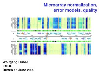
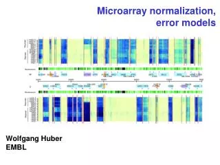
Effect on Spatial Artifacts Median normalization Global lowess normalization Scaled Print-tip normalization Print-tip lowess normalization
Quantile Normalization • Determine reference distribution (can use any good chip or average a set of chips) • For each chip, for each probe, determine quantile within that chip • Shift to corresponding quantile of reference distribution ---------------------------------- • Easy to implement • Resolves intensity dependent bias as well as loess
Quantile Normalization (Irizarry et al 2002) The mapping by quantile normalization
THINGS TO MAYBE ADD • Maybe examples of how to do mapping • How to assign reference • linear extension to high genes • Critiques: induced correlations –example and details about variable cross-hybe
Key Assumption of Quantile Norm • The processes that distort the distribution act on all probes of a given intensity more or less equally • Probably true within differences of 30% or 40% • Smaller differences depend quite strongly on technical characteristics of probes
Critiques of Quantile Normalization • Artificially compresses variation of highly expressed genes • Confounds systematic changes due to cross-hybridization with changes in abundance to genes of low expression • Induces artificial correlations in gene expression across samples
How to Assess Normalization? • We want to minimize technical variations in relation to biological variation • Most tests like t-test or ANOVA compare technical and between-group variance • Compare distributions of biological to technical variation after normalization • Most small estimates of variance are under-estimates
Other Issues in Normalization • Transformation of variables • Variance stabilization • Background compensation
Why Variance Stabilization? x-y plot mean-var plot Ideal raw x log2 (x) log2 (x+offset) From Du CHI 2007
Variance Stabilization • Simple power transforms (Box-Cox) often nearly stabilize variance • Durbin and Huber derived variance-stabilizing transform from a theoretical model: • y = a (background) + m eh (mult. error) + e (static error) • m is true signal; h and e have N(0,s) distribution • Transform: • Could estimate a (background) and sh/se empirically • In practice often best effect on variance comes from parameters different from empirical estimates • Huber’s harder to estimate
Model Solution – arcsinh Fit the relations between mean and standard deviation Relations between log2 and VST (arcsinh) (Lin, Pan, Huber, and Warren, 2007)
Oligonucleotides (50-mers) immobilized on glass beads Identifier tag on each oligo Usually ~ 30 beads per probe Illumina Bead Arrays
Comparing VSN results with log scale MAQC data VST improves the cross-site concordance From Du CHI 2007
Applicability to Other Array Types • The crucial assumption of most current methods for expression array normalization is that the differences between arrays reflect changes in only a small proportion of the genome and that the overall distribution of expression levels is unchanged
Recent Approaches • Use of standard or control variables to infer covariates Mike West • PCA of residuals to infer covariates or patterns of systematic error • Regression on technical covariates of probes
Inferred (Surrogate) Covariates • Surrogate variable analysis (SVA) • Leek and Storey, PLoS Genetics, 2007 • Motivation: many unmodeled (and unknown) factors affect the measures • Even if known, most experiments don’t have sufficient d.f. to estimate their effects • Idea: often the effects of all factors are somewhat correlated • Can you infer a manageable set of ersatz (surrogate) covariates that do the same thing?
Underlying Model • There are factors f1, …, fL, which affect genes via linear combinations of functions gi1(f1), …, giL(fL). • The distorting effect on gene i in array j is: • Claim: this is a sufficiently general representation, because additive models can represent most data sets (dubious) • Fact: an additive representation can be represented as a linear function (of transformed variables)
Inferring Covariates • Given observations Y and predictors XL x N , • (e.g. X might record diagnosis and age in columns) • Fit the following model: • The residual matrix R is approximated by R ~ ULVT using singular value decomposition with K non-trivial components • The kth row of matrix V records the kth inferred covariate across the N samples
How many singular values to keep? Test whether fraction of variance explained higher than ‘chance’ Compute test statistic Assess significance by SVD following many permutations, acting on rows independently, to disrupt correlation structure SV Decomposition of Residuals Surrogate variables
Using the Surrogate Covariates • For each gene i separately fit b’s and l’s in model: • Issue: How to limit d.f. used up by covariates? • For each k, many genes show little correlation with inferred covariate k. • Compute variance explained by each covariate across all genes • Select which genes i are significantly associated with predictor vk .(i.e. lik > 0) using Storey’s FDR approach on variance explained • Include only those significantly associated
Critiques and Issues for SVA • SVA does not distinguish between technical variation and biological variation in most designs • Biological variation within treatment groups is often important • SVA assumes covariate effects are additive (linear in practice) • This may be plausible for a single outcome, but the assumption of the model is that the same functions of the unknown factors contribute linearly to the distortion of ALL genes • Fairly complex procedure with several tuning parameters • Does not address confounding between systematic errors and design • a general fault of covariate methods, but not (I think) necessary • SVA as published is not robust – easily fixed
Left singular vectors represent basis for subspace of technical variation Hypothesis: Technical errors are reproducible Implication: one can ‘learn’ typical patterns of technical variation for each technology from one set of replicates A Simpler Approach Using SVD
Algorithm • Consider sets of technical replicates of the same samples, with only technical differences within sets • PCA of replicates identifies major components • Algorithm: • Construct technical differences from mean of each set • Robust PCA of differences • Outliers can be handled by simple winsorization • Find differences of each array from common mean of all arrays in experiment • Project each array’s difference onto K PC’s (K small) • Subtract projection (typically 50% of variance) • Leverage points in regression are also winsorized
Principal Components of MAQC • Four samples: A: brain; B mixed tissue; C: 3:1 mixture of A & B; D 1:3 mixture of A & B • Each sample hybridized five times in each of three labs Scree plot of replicate PCA for Agilent 44K 1 color MAQC data set (3 sets of 4x5 reps)
Using each lab’s PC’s to normalize the other two labs Five PC’s (left singular vectors) used Proportion of variance explained > 50% 5/40,000 expected if taking a ‘random’ subspace Results on MAQC Data Number of F-scores greater than 7
Technical Variable Regression • Hypothesis: • Most technical variation between chips is caused by a few (unknown) systematic factors • Probes with similar technical characteristics (Tm, position in gene, location on chip, typical intensity, ..) will be distorted by similar amounts • Therefore we can use technical variables as an index of technical similarity (the predictor) and (usually) treat real biological differences as ‘noise’ • Construct deviations from average or standard chip • Identify which technical variables have the most effect • Regress deviations from average on technical variables
Covariates to Index Similar Probes • Analogous to ‘loess’ normalization of Yang et al • Index similar probes by technical covariates • Known covariates of array probes • Location (X,Y) on chip • Reference (or average) intensity • Tm (‘melting’ or annealing temperature) • Location relative to priming site • for expression arrays • Pyrimidine content (C + T) • Cross-hybridization easier than with purines • Deviation of reference from average reference (two color arrays) Deviations of log intensity from average as function of average
Many Covariates Predict Deviations • A moderate number (5-9) of technical predictors have significant effects on many chips • Non-linear, non-additive interactions are usual LOESS curves tracking: Low CT; near 3’ end Deviations of chip GSM 25410 from average of all chips in expt. Overall downward trend (apparent loss of expression) at higher values of average intensity High CT; near 3’ end Low CT; far 3’ end High CT; far 3’ end Average of all chips
Regression in Moderate Dimensions • Local regression (LOESS) works reasonably well up to three or four dimensions, but there is too much flexibility in five or more dimensions • Curse of dimensionality: If 7 variables are truly independent at all levels, and if 4 bins for each variable: 47 = 16,384 bins • But there is plenty of data! • How to reconcile flexibility with restricting df? • Representation: How to represent the high-dimensional surface effectively for 105 points?
Addressing Curse of Dimensionality • Local regression unwieldy in 7 dimensions • There don’t seem to be dimension reduction subspaces within predictors • The condition number of the data matrices selected by 5% ‘slices’ is 1.5 - 2 • Approaches such as MARS don’t seem to work, because interactions dominate most main effects • Manufacturers tune the probes to remove main effects
Issues in Building Representation • Spend degrees of freedom wisely • Borrow idea from MARS – limit number of effective dimensions in local regression • Construct neighborhoods in B7 that are wide in most directions, but narrow in directions of high variation • Directions determined adaptively with high threshold