Download

1 / 84
840 likes | 983 Views
Microarray Pre-processing, quality control and normalization. Practical Problems 1. Comet Tails Likely caused by insufficiently rapid immersion of the slides in the blocking solution. Practical Problems 2. Practical Problems 3. High Background 2 likely causes: Insufficient blocking.

E N D
Microarray Pre-processing, quality control and normalization
Practical Problems 1 • Comet Tails • Likely caused by insufficiently rapid immersion of the slides in the blocking solution.
Practical Problems 3 High Background • 2 likely causes: • Insufficient blocking. • Precipitation of the labeled probe. Weak Signals
Practical Problems 4 Spot overlap: Likely cause: too much rehydration during post - processing.
Practical Problems 5 Dust
Steps in Images Processing 1. Addressing: locate centers 2. Segmentation: classification of pixels either as signal or background. using seeded region growing). 3. Information extraction: for each spot of the array, calculates signal intensity pairs, background and quality measures.
Steps in Image Processing 3. Information Extraction • Spot Intensities • mean (pixel intensities). • median (pixel intensities). • Pixel variation (IQR of log (pixel intensities). • Background values • Local • Morphological opening • Constant (global) • None • Quality Information Signal Background
Addressing This is the process of assigning coordinates to each of the spots. Automating this part of the procedure permits high throughput analysis. 4 by 4 grids 19 by 21 spots per grid
Addressing Registration Registration
Problems in automatic addressing Misregistration of the red and green channels Rotation of the array in the image Skew in the array Rotation
Segmentation methods • Fixed circles • Adaptive Circle • Adaptive Shape • Edge detection. • Seeded Region Growing. (R. Adams and L. Bishof (1994) :Regions grow outwards from the seed points preferentially according to the difference between a pixel’s value and the running mean of values in an adjoining region. • Histogram Methods • Adaptive threshold.
Limitation of fixed circle method SRG Fixed Circle
Limitation of circular segmentation • Small spot • Not circular Results from SRG
Information Extraction • Spot Intensities • mean (pixel intensities). • median (pixel intensities). • Background values • Local • Morphological opening • Constant (global) • None • Quality Information Take the average
Quality Measurements • Array • Correlation between spot intensities. • Percentage of spots with no signals. • Distribution of spot signal area. • Spot • Signal / Noise ratio. • Variation in pixel intensities. • Identification of “bad spot” (spots with no signal). • Ratio (2 spots combined) • Circularity
QC implementation • marray and arrayQuality packages in Bioconductor (R) can help identify dye, hybridization and other experimental artifacts • Bioconductor: http://www.bioconductor.org/ • R: http://www.r-project.org/
Why Normalization? • Many sources of systematic variation that affect measured gene expression. • Differences in labeling efficiency of red and green dyes • Print-tip effects • Array batch effects
Within-Slide Normalization • Normalization balances red and green intensities. • Imbalances can be caused by • Different incorporation of dyes • Different amounts of mRNA • Different scanning parameters • In practice, we usually need to increase the red intensity a bit to balance the green
Methods? log2R/G -> log2R/G - c = log2R/ (kG) Standard Practice (in most software) c is a constant such that normalized log-ratios have zero mean or median. Speed Approach: c is a function of overall spot intensity and print-tip-group. What genes to use? • All genes on the array • Constantly expressed genes (house keeping) • Controls • Spiked controls (e.g. plant genes) • Genomic DNA titration series • Other set of genes
Experiment Probes: ~6,000 cDNAs, including 200 related to lipid metabolism.
M vs. A M = log2(R / G) A = log2(R*G) / 2
Normalization - Median • Assumption: Changes roughly symmetric • First panel: smooth density of log2G and log2R. • Second panel: M vs. A plot with median set to zero
Normalization - lowess • Global lowess • Assumption: changes roughly symmetric at all intensities.
Normalisation - print-tip-group Assumption:For every print group, changes roughly symmetric at all intensities.
Within print-tip-group box plots forprint-tip-group normalized M
Taking scale into account Assumptions: • All print-tip-groups have the same spread. True ratio is mij where i represents different print-tip-groups, j represents different spots. Observed is Mij, where Mij = aimij Robust estimate of ai is MADi = medianj { |yij - median(yij) | }
Paired-slides: dye swap • Slide 1, M = log2 (R/G) - c • Slide 2, M’ = log2 (R’/G’) - c’ Combine bysubtracting the normalized log-ratios: [ (log2 (R/G) - c) - (log2 (R’/G’) - c’) ] / 2 [ log2 (R/G) + (log2 (G’/R’) ] / 2 [ log2 (RG’/GR’) ] / 2 provided c = c’ Assumption: the separate normalizations are the same.
Summary Case 1: A few genes that are likely to change Within-slide: • Location: print-tip-group lowess normalization. • Scale: for all print-tip-groups, adjust MAD to equal the geometric mean for MAD for all print-tip-groups. Between slides (experiments) : • An extension of within-slide scale normalization (future work). Case 2: Many genes changing (paired-slides) • Self-normalization: taking the difference of the two log-ratios. • Check using controls or known information.
A probe set = 11-20 PM,MM pairs There may be 5,000-55,000 probe sets per chip
Chip QC: Defect Classes • In order of occurrence: • Dimness • High Background • Unevenness • Spots • Haze Band • Scratches • Brightness • Crop Circle • Cracked • Snow • Grid Misalignment • Training set of 7K chips (Human, Rat, Mouse)