Download

1 / 26
280 likes | 556 Views
Microarray data normalization and data transformation. Ka-Lok Ng Asia University. Estimating background. http://www.mathworks.com/company/pressroom/image_library/biotech.html.

E N D
Microarray data normalization and data transformation Ka-Lok Ng Asia University
Estimating background http://www.mathworks.com/company/pressroom/image_library/biotech.html • Reference: Causton H., Quackenbush J., and Brazma A. Microarray Gene Expression Data Analysis. A Beginner’s Guide, Ch.3, Blackwell (2003) • most image processing software reports background subtracted values for each feature (spot) on the array by first estimating the background and then subtracting it pixel by pixel. • Local estimate of the background by identifying some number of pixels surrounding each spot and using those to calculate an average or median background level that can be subtracted from each pixel in the spot. • Disadvantage – if the pixels selected contain portions of the target spot, one may overestimatethe background significantly • Some image processing software allows the estimation of global background – a single measurement that is used for the entire slide. This requires users to select a large representative area of the slide that is devoid of features. • Disadvantage – it fails to account for local variation in the background fluorescence of the substrate, and as result it may provide either an over- or underestimate of the appropriate background.
Estimating background Reference: Baxevanis A. and Ouellette B.F. Francis. Bioinformatics Ch. 16. J. Wiley (2005) There are a number of schools of thought regarding the estimation of background for DNA microarrays (1) Not to calculate a background value • But rather to try to estimate it using statistical techniques • Argument – subtracting background introduces significant variance into the estimation of hybridization intensity, decreasing the reliability • Although this may not produce any significant changes in relative expression levels between conditions for highly expressed genes, it can have profound effect on estimates for genes expressed at low to moderate levels (2) Chooses to subtract background • To use the fluorescence of the area surrounding each feature on the array. It uses the ‘naked’ substrate (where no DNA is spotted) to estimate the background for features that contains DNA, and as such neglects contributions from nonspecific hybridization (i.e. unwanted signal) • An alternative – use negative control features printed on the array, these may provide an estimate of nonspecific hybridizatoin, but there may not have enough features (spots) on the array to provide an estimate of local background variation
Gene expression ratio • Most analysis focus on differences in gene expression, which are reported as a background subtracted ratio of expression levels between a selected query sample and a reference sample. • It is done by taking ratios of the measured expression between two physical states for each gene k on the array, where one designated the query and reference samples R and G respectively.
Gene expression ratio • A variety of methods for calculation the expression ratio using the median, mean and integrated expression measures. If we choose to measure expression using the median pixel value for each feature, then the medianexpression ratio for a given feature is where and are the median intensity values measured for pixels identified in the feature (gene) and background respectively.
Transformation of the gene expression ratio • Ratios are useful because they allow us to measure expression differences in an intuitive way • However, ratios are troublesome because they treat up- and down regulated genes differently. Genes up-regulated by a factor of 2 have an expression ratio of 2, while those down-regulated by a factor of 2 have an expression ratio of ½. As result, down-regulated genes are compressed between 1 and 0, while up-regulated genes expand to cover the region between 1 and positive infinity. • A better alternative is to apply a logarithmic transformation, generally using the logarithm base 2. the advantage of this transformation is that it produced a continuous spectrum of values for differentially expressed genes while treating up- and down-regulated genes equivalently. • log24 = 2, log2¼ = -2 • Disadvantage ratio remove absolute gene expression information
Experimental errors Situation where expression does not correlate with spot intensity • Image processing gives poor estimationof the mean, median or total intensities • Pixel saturation • Background estimation • Density of fluors in the labeled hybridized molecules is high enough, interaction between the dye molecules can quench fluorescence • Poor labeling or hybridization can result in signals too faint to allow detection of certain expressed genes • Significant cross-hybridization • PCR oligonucleotides may be contaminated with other DNAs and may not bind with only the gene of interest • Oligonucleotide sequences may be incorrectly synthesised • Hybridization between alternative splice forms and members of gene families may cause overestimate fluorescence and therefore expression • Sample handling problems – hypoxia (缺氧), cold, heat shock or cell death of tissue samples can cause genes to be expressed that are not normally present in the tissue we want to study • RNA degradation can skew representation, as some RNAs are more stable than others the best protection against any of these artifacts is to institute validated laboratory protocols The signal for each gene is due to a combination of the hybridization of that gene + some non-specific hybridization, from all the other similar sequences, or partial transcripts in the sample, plus noises.
Normalization of gene expression • A variety of reasons why the raw measurements of gene expression for two samples (query and reference) may not be directly comparable • Quantity of starting RNA, [RNA]target ≠ [RNA]sample • Difference in Cy3 and Cy5 labeling • Difference in Cy3 and Cy5 detection efficiencies (i.e. laser absorption efficiency) Consider a self-self comparison in which the same sample is compared with itself expectsthe measured log2(ratio=R/G) to be 0 for each gene • However, typically these are found to be distributed with a non-zero mean and standard deviation, indicating that there is a bias to one sample or the other • Normalization is any data transformation that adjusts for these effects and allows the data from two samples to be appropriately compared. • Normalization scales one (R or G) or both (R and G) of the measured expression levels for each gene to make them equivalent, and the expression ratios derived from them
Normalization of gene expression Data normalization • Assume data have already sorted and there are no data missing (delete or by interpolation『數學』以插值法求值) • Data normalization the process of correcting two or more data sets prior to comparing their gene expression values • the background intensity signal (noise) is measured and subtracted from the Cy3 and Cy5 chs (background may be constant or it may vary locally) • apply a local orglobal normalization (such as overall average) to raw measurements (such as ratio (G/R) or Log2 (Log2(G) – Log2(R) transformed) • Other global normalization method choose a set of housekeeping genes (commonly expressed across all tissues, such as the Human Gene Expression (HuGE) index database http://www.biotechnologycenter.org/hio/
Total intensity normalization • Assuming [total RNA]target = [total RNA]sample, same total intensity • [Red]target = [Green]sample • Under this assumption, a normalization factor can be calculated and used to rescale the intensity for each gene in the array • Assume that the arrayed elements represent a random sampling of the genes in the organism no oversample or undersample the genes in the query or reference sample no bias • The normalization factor Ntotal is calculated by summing the measured intensities in both channels where Gk and Rk are the measured intensities for the kth array feature (such as the Cy3 and Cy5 intensities) and Narray is the total number of genes in the microarray, the summation runs over the subset of genes selected as normalization standards.
Total intensity normalization • The intensities are rescaled such that Gknormal = Ntotal Gk and Rknormal = Rk and the normalized expression ratio for each feature becomes which adjusts the ratio such that the mean ratio is equal to 1, this transformation is equivalent to subtracting a constant from the logarithm of the expression ratio log2(Tknormal) = log2(Tk) – log2(Ntotal) • Disadvantage of total intensity normalization – insensitive to systematic variation in the log2(ratio)
Scatter plot analysis • A scatter plot analysis of the raw Cy3 and Cy5 values of all the 6912 elements within the 5 gene clusters is shown in the figure on the right (4 plots). • The top two plots represent all the elements and the bottom two depict the genes that show the largest differences in signal. • Most of the genes that are distinct between the samples are expressed at lower levels (low fluorescent signal). These differences were more exaggerated in the aRNA than the mRNA sample because the signal-to-noise ratio was typically much greater in the aRNA sample. http://www.ambion.com/techlib/tn/95/954.html
Scatter plot of Cy5 and Cy3 Scatter plot of Cy5 and Cy3 • It is expect that the Cy5 and Cy3 plot should fall on the diagonal (i.e. Cy5 = Cy3) • In this plot, most of the points are found below the diagonal suggesting that for most of the points, the values measured on the Cy3 ch are higher than the values measured on the Cy5 ch. • Two possible caused, (1) either the mRNA labelled with cy3 wasmore abundant for most of the genes or (2) the cy3 dye more efficient for the same amount of mRNA, i.e. cy3 tends to have a stronger intensity http://molas1.nhri.org.tw/~molas/index.htm?item=example&subitem=analysis-2&PHPSESSID=718975800da6f79d287871e77f50b33a
Scatter plot of Cy5 and Cy3 data Raw data Normalize data
Stanford MicroArray Database • http://genome-www5.stanford.edu/ • To download the yeast cell cycle time series data • Public login go to “Select arrays by Experimenter, Category, Subcategory and Organism” page, • set experimenter=Spellman, Category=cell cycle press ‘display data’ select alpha factor release sample013 raw data set decompress the Excel file
alpha factor release013 raw data How the microarray date are represented • Ch1 Intensity (Mean) Ch1 Net (Median) Ch1 Intensity (Median) % of saturated Ch1 pixels Std Dev of Ch1 Intensity ch 1 Background (Mean) Ch1 Background (Median) Std Dev of Ch1 Background Ch1 Net (Mean) • Ch2 Intensity (Mean)Ch2 Net (Mean) Ch2 Net (Median) Ch2 Intensity (Median) % of saturated Ch2 pixels Std Dev of Ch2 Intensity ch 2 Background (Mean) Ch2 Background (Median) Std Dev of Ch2 Background • Ch2 Normalized Background (Media) Ch2 Normalized Net (Mean) Ch2 Normalized Intensity (Mean) Normalized Ch2 Net (Median) Normalized Ch2 Intensity (Median) Regression Correlation Diameter of the spot Spot Flag • Log(base2) of R/G Normalized Ratio (Mean)Log(base2) of R/GNormalized Ratio (Median) R/G Mean (per pixel) R/G Median (per pixel) % CH1 PIXELS > BG + 1SD % CH1 PIXELS > BG + 2SD % CH2 PIXELS > BG + 1SD % CH2 PIXELS > BG + 2SD G/R (Mean) • G/R Normalized (Mean)R/G (Mean) R/G (Median) Std Dev of pixel intensity ratios R/G Normalized (Mean) • Ch1 Net (Mean) = Ch1 Intensity (Mean) - Ch1 Background (Median) • Ch2 Net (Mean) = Ch2 Intensity (Mean) – Ch2 Background (Median) • Ch2 Normalized Net (Mean) = Ch2 Normalized Intensity (Mean) - Ch2 Normalized Background (Media) • R/G (Mean) = Ch2 Net (Mean) / Ch1 Net (Mean) = 1/ [G/R (Mean)] 5. R/G Normalized (Mean) = Ch2 Normalized Net (Mean) / Ch1 Net (Mean) = 1/ [G/R Normalized (Mean)] 6. Log(base2) of R/G Normalized Ratio (Mean) = Log [R/G Normalized (Mean)]
alpha factor release013 raw data • column M is the ORF Name • Column O = Sequence Type = control, AORF or ORF • Box AV94 Ch1 Net (Mean) is an empty entry Ch1 Intensity (Mean) Box AN94 = 264, Ch1 Background (Median) Box AT94 =280, because 264 – 280 < 0 !!
Data Normalization • An extreme example
Lowess normalization • It is noted that in a number of reports that the log2(ratio) values often have a systematic dependence on intensity, most often a deviation from 0 for low intensity spots. • Lowess normalization – a method that can remove intensity-dependent dye-specific effects in the log2(ratio) values Method • Plotting the measured log2(R/G) ratios for each array feature as a function of the log10(R*G) or ½*log2(R*G) product intensities. The resulting ‘R-I’ (for ratio-intensity) can reveal intensity-specific artifacts (人工作品) in the measurement of the ratio. • Self-self hybridization test - It is expect to see absolutely no differential expression and consequently all log2(ratio) measures should be zero on average. • The R-I plot shows a slight downward and upward curvature at the low and high intensities ends respectively, as well as an increased spread in the distribution of log2(ratio) values at low intensities. • Lowess corrects these by performing a local weighted linear regression for each data point in the R-I plot and subtracting the calculated best-fit average log2(ratio) from the experimentally observed ratio for each point as a function of the log10(intenisty). An R-I plot displays the log2(Ri/Gi) ratio for each element on the array as a function of the log10(Ri*Gi) product intensities and can reveal systematic intensity-dependent effects in the measured log2(ratio) values. Data shown here are for a 27,648-element spotted mouse cDNA array. http://www.nature.com/ng/journal/v32/n4s/fig_tab/ng1032_F1.html Application of local (pen group) lowess can correct for both systematic variation as a function of intensity and spatial variation between spotting pens on a DNA microarray. Here, the data from Fig. 1 has been adjusted using a lowess in the TIGR MIDAS software (with a tri-cube weight function and a 0.33 smooth parameter) available from http://www.tigr.org/software. See http://www.nature.com/ng/journal/v32/n4s/fig_tab/ng1032_F2.html
Lowess normalization Local variation as a function of intensity can be used to identify differentially expressed genes by calculating an intensity-dependent Z-score. In this R-I plot, array elements are color-coded depending on whether they are less than one standard deviation from the mean (brown), between one and two standard deviations (blue), or more than two standard deviations from the mean (green). http://www.nature.com/ng/journal/v32/n4s/fig_tab/ng1032_F4.html
Lowess normalization • Lowess detects systematic deviations in the R-I plot and corrects them by performing a local weighted linear regression as a function of the log2(intensity) and subtracting the calculated best-fit average log2(ratio) from the experimentally observed ratio for each data point. • If one sets Lowess estimates y(xi), the dependence of the log2(ratio) on the log2(intensity),and then uses this function, point by point, to correct the measured log2(ratio) values, so that after Lowess correction
Data filtering Why do we need data filtering ? • Filter the dataset to reduce its complexity and increase its overall quality What kind of data are filtered ? • Low quality data – filtering low and high intensity data Filtering low intensity data • By examining several representative R-I plots, it is obvious that the variability in the measured log2(ratio) values increases as the measured intensity decreases • This is because relative error increases at lower intensity (relative error = error/(raw intensity),↑as raw intensity↓) • Good elements would have intensities more than two standard deviations above background. Only spots where the measured signals meet the criteria that and similarly for the mean. Other approaches include the use of absolute lower thresholds for acceptable array elements (sometimes referred to as “floor”) or percentage-based cutoffs in which some fixed fraction of elements is discarded.
Data filtering Filtering high intensity data • At the high end spectrum, the array elements saturate the detector used to measure fluorescence intensity • As soon as the intensity approaches its maximum value (typically 216 – 1 = 65535/pixel for a 16-bit scanner), comparisons are no longer are meaningful, because the array elements become saturated and intensity measurements cannot go higher. • There are a variety of approaches to dealing with this problem as well, including eliminating saturated pixels in the image-processing step or setting a maximum acceptable value (often referred to as ceiling) for each array element.
Use of replicate data • Replication is essential for identifying and reducing the effect of variability in any experimental assay Two broad classes • Biological replicates use independently derived RNA from distinct biological sources to provide an assessment of both the variability in the assay and the biological sample • Technical replicates use repeated measurements of the same biological samples, which provide only information on the variability of the spots. These include • Printing exactly the same DNA at different locations on the same slide control the noise introduced by the location of the spot on the slide (could be affected by local defects !) • Print several exact copies and hybridize several times with exactly the same mRNA in exactly the same conditions control the noise introduced by the hybridization stage
Exercise Calculate the net intensity, normalize net intensity, R/G, normalize R/G ratio for ch 1 (green) and ch 2 (red) respectively
SMD data analysis – Hs. Primary liver tumor Scatter plot • Raw plot ch 2 Intensity vs. ch 1 Intensity • Normalize plot ch 2 Normalize (mean) vs. ch 1 net (mean) Lowess plot • Raw plot Log2 (ch 2 Int./ch 1 Int.) vs. Log10(ch 1 Int. * ch 2 Int.) • Normalize plot Log2[normalize (R/G)] vs. Log10[(ch 1 net (mean) * ch 2 normalize net (mean))]