CONCLUSIONS

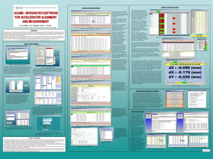
1. Figure 18 – Capture Interface – Real Time Positioning (RTP) View Figure 3 – Stand Alignment (step 1) Option For step 1 projects, the user can simply enter a centrally located stand, or control monument, and the program will check through a database of stand or pedestal coordinate data. All the relevant components are then displayed in the right hand list box, and available monuments in the localized area are displayed in the left box. The user can then pick and choose which information to include in the project. Figure 11 – Common Interface – Resected Theodolite Tab View Figure 5 – Spectrometer Alignment Option Figure 5 illustrates how a spectrometer survey is undertaken. All information is pre-determined, and rapidly added to the project information. Figure 6 – Standard Project Information Screen Project information is added to the job files with this screen. Every style of project uses this common menu. Fig. 23 – Weight Observations Option 1 Figure 25 – Weight Coordinates Option Fig. 24 – Weight Observations Option 2 Capture Interface Outline Common Interface Outline Theodolite data collection takes place using the capture interface screens. Figure 14 shows the main data capture screen. Upon switching from the common interface via the resume or new position commands, all available serial ports are automatically sensed to see what theodolites are attached and a display such as figure 14 comes up. Targets that have both a forward and reverse observation are highlighting by having the cell containing the station name turn green. Observation pairs which do not meet the 2 face tolerance limits have their cells that display the angles highlighted in bright red. Distances can be observed, and there are options to add standard prisms plus meteorological data. The common interface is where most details about a project are located. Users can use a variety of commands to navigate throughout ACAMS. Figure 7 illustrates the control point information. From this tab, users can see what weights have been assigned to each control point, and adjust the point accordingly if the situation required such action. This commonly occurs with vertical point information in Jefferson Lab’s Experimental halls, as the Spectrometers are frequently moved to various angles, causing localized deflections of the hall floor. Figure 7 – Common Interface – Control Tab View Abstract ACAMS (Accelerator Combined Alignment and Measurement System) is a software package that has been developed at Thomas Jefferson National Accelerator Facility (Jefferson Lab). ACAMS was developed to replace four dos based software programs. These programs operated independently and all used theodolite observations as the common basis for data collection. The methodology used to collect the data was similar, but there were inconsistencies and shortcomings in these processes. ACAMS now integrates all the reductions, adjustment and reporting into one package. Jefferson Lab Alignment group now relies on ACAMS for most of the field surveys undertaken. Many new features that were lacking in the older packages have been included in the development of ACAMS. This paper will discuss the reasoning behind the development, current available features, and the future direction that the software will take.  This work was supported by the United States Department Of Energy under contract number DE-AC05-84ER40150. Figure 8 illustrates the target point information. In this particular example, the design z,x,y coordinates and the resulting information from an adjustment are shown (as the found z,x,y coordinates). The differences between the design coordinates and the surveyed coordinates are displayed as dz,dx,dy. The adjustments standard error information is also displayed. Users can save any set of data to a report template, which allows as-found information to be stored. If components need to be monitored during the project, any set of coordinates may be saved and added to the report, using this utility. There is a facility to toggle between the ‘grid coordinates’ and the ‘beam following’ (bfs) which aids the crew in setting components. Figure 15 shows the observation tabulator. This popup screen allows the user to see which targets or control points have been observed at the various theodolite stations. It displays whether a point has been observed with both faces (displays a ), single face (½), or not at all (shows a X) for each station. Figure 14 – Capture Interface – Main Observation Collection View Figure 15 – Observation Tabulator Figure 16 illustrates the ‘Display Movement’ command view. Users can choose between displaying the difference between either ‘movements’ to set a particular component or the actual ‘location’ of the component. Information showing the standard errors of the target point is also presented. A additional feature currently being developed, is to tie our fiducial database to the located components and then calculate the reverse least squares transformation to find the component center and rotation values. This information will be displayed in this screen. Figure 17, shows the options available from one of the pull-down menus in the Capture Interface. From the ‘Calculate’ command, the users can run a variety of fitting routines, distance calculations or other various commands. Project Type Options Figure 17 – Calculate Options Figure 8 – Common Interface – Target Points Tab View Figure 16 – Capture Interface – Movements Display View Figure 9 shows the raw field data information. All information recorded when the data was taken is stored in the raw file. Users can tab between any of the set position / theodolite combinations. No editing of observations is allowed. Options exist in the data capture section, which allow individual observations to either be deleted or re-observed. One of the main features available in ACAMS is the Real Time Positioning (RTP) routine. This routine is used to position any object into its desired alignment. The procedure requires the crew to observe the control points, the components to be aligned, and obtain an adjustment from 3DCD. They can then use the ‘RTP Toggle’ option on the main data capture toolbar. This then takes the program to a new screen, figure 18, where the theodolites are polled at either set time intervals or the instrument operators take manual observations, to align a component to any given set of design coordinates.  As the instrument operators take observations, the coordinates are automatically updated, using a least squares solution. A value, based upon the original forward and reverse observations taken to the targets, is used to correct single face observations taken in RTP. The input file to 3DCD is updated with the corrected angles, and after the adjustment, the differences between design and the presently located target are calculated. The differences are then displayed as shown in figure 18, and the crew can make the necessary adjustments to the component, and iterate until the component is within an acceptable tolerance. After adjusting all the required elements by using the RTP routine, the crews will lock-down the elements and conduct a final survey using forward and reverse observations. Figure 1 – Project Type Selection Menu Operators must choose from the list of options as shown in figure 1. There are 4 main options which start new survey projects. They are, ‘New Fiducial File’, Step 2 (magnet alignment), Step 1 (stand alignment) or Spectrometer surveys. Additional options are for appending or resuming a project, using an existing control file to start a new project, choosing to open a project which wasn’t the last, or importing project control and target information. Figure 2 – Fiducialization Option This option illustrates the menu available when fiducializing objects. Users can generate a group of points and Theodolite ID tags (numeric) at this point. Groups of points can automatically be generated. Scale bars are also numerated at this point. Figure 9 – Common Interface – Raw Observations Tab View Figure 10 illustrates the report building facility. Users can use the options available here to build custom reports. Final standard reports can automatically be created when a project is exited. An illustration of a partial report from a Step 2 alignment is shown in figure 12. Spectrometer Alignment Options Jefferson Lab’s Hall A contains two high resolution spectrometers and Hall C has a High Momentum (HMS) and a Short Orbit (SOS) spectrometer. All four spectrometers rotate about a central target. The alignment group is frequently called upon to determine the angle between the incoming beam and the centerline of the spectrometers. ACAMS is used to survey the spectrometer with respect to the local monuments. After a satisfactory adjustment with 3DCD, the results are processed using transformation software to determine the central axis of the spectrometers with respect to the beam. ACAMS automates this process resulting in smooth flow of information between processes. Figure 19 shows the options that the crew steps through to calculate the desired spectrometer angle. Shown in figure 20 is the output from a Hall A Electron spectrometer survey. All the information required by the physicist is contained in this output. Figure 4 – Magnet Alignment (step 2) Option Figure 4 displays 2 screens that users navigate through when conducting Step 2 style surveys. The top illustration shows how the Lab’s accelerators are sectionalized into areas, which are again broken into sectors within each area. Individual component information is then available to the users to select from each sector. Finally, individual targets on the components can be selected. The second portion of the illustration, shows the auto-numbering and editing facility available to the users. Figure 10 – Common Interface – Report Builder Tab View Figure 19 – Spectrometer Alignment Commands Figure 20 – Spectrometer Angle Results The final available tab screen in the common interface is for theodolite information. Figure 11 illustrates the information available to the users. Theodolite coordinate standard error information, plus the rotational values that resulted from the least squares adjustment is displayed. Adjustment Details Figure 21 displays the results from 3DCD, a least squares bundle adjustment (originally developed at Stanford Linear Accelerator). 3DCD has been optimized to accept any size arrays, and made into a windows DLL. This screen summarizes the corrections calculated during the adjustment and the final resulting standard error, iterations and degrees of freedom. Figure 22 illustrates the various views that can also be shown from this section of the program. View options are capable of displaying the input file, adjusted coordinate file, total adjustment output, theodolite information, and raw observations file. Figures 23 to 25 show the weighting options that are available to the users. Entire sets of observations from a particular theodolite location can be weighted out from the adjustment from figure 23. Figure 24 illustrate how users can weight individual observations; they can also order the observations by largest residuals. Figure 25, shows how users can alter the weights on the control points. Figure 13 shows the popup screen that appears, upon completion of a project. Users can select which files to send to a floppy disk. Certain files are automatically checked for upload, but the user can select more or less, as the situation may require. Figure 21 – Adjustment Results Summary Screen Figure 22 – Adjustment View Options Screen CONCLUSIONS With approximately a half man-years of coding investment, ACAMS has combined several disjointed field operations and procedures into a tightly integrated operation. Additions have been made to the software, which have provided several new and valuable tools to the users. The crews have commented on the software’s ease of use, the ability to rapidly align components, and conduct other essential alignment tasks. ACAMS was developed in order to integrate Jefferson Lab’s existing theodolite based alignment software into one package. ACAMS is now the main tool used by the Alignment Group. The software has given Jefferson Lab a tool that fits it requirements, and traditional alignment operations while also allowing the group to have the flexibility and control over its development as circumstances dictate. Future development that includes integration of updated and new equipment, and the ability to customization the software to specific tasks should make ACAMS a tool that will be used at the lab for many years. I would like to thank and recognize the alignment group at the Stanford Linear Accelerator for supplying the original code for the bundling program 3DCD, and a particular thanks to Catherine Le Cocq for the use of the WINFIT program. A special thanks also goes out to all the field staff at the lab for their patience, suggestions and verification of all the processes developed for ACams. Figure 13 – File Transfer Figure 12 – Final Report on Exit