Download
1 / 59
610 likes | 886 Views
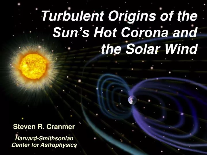
Turbulent Origins of the Sun’s Hot Corona and the Solar Wind. Steven R. Cranmer Harvard-Smithsonian Center for Astrophysics. Turbulent Origins of the Sun’s Hot Corona and the Solar Wind. Outline: Solar overview: Our complex “variable star” How do we measure waves & turbulence?

E N D
Turbulent Origins of the Sun’s Hot Corona andthe Solar Wind Steven R. CranmerHarvard-SmithsonianCenter for Astrophysics
Turbulent Origins of the Sun’s Hot Corona andthe Solar Wind • Outline: • Solar overview: Our complex “variable star” • How do we measure waves & turbulence? • Coronal heating & solar wind acceleration • Preferential energization of heavy ions Steven R. CranmerHarvard-SmithsonianCenter for Astrophysics
Motivations for “heliophysics” • Space weather can affect satellites, power grids, and astronaut safety. • The Sun’s mass-loss & X-ray history impacted planetary formation and atmospheric erosion. • The Sun is a unique testbed for many basic processes in physics, at regimes (T, ρ, P) inaccessible on Earth . . . • plasma physics • nuclear physics • non-equilibrium thermodynamics • electromagnetic theory
The Sun’s overall structure • Core: • Nuclear reactions fuse hydrogen atoms into helium. • Radiation Zone: • Photons bounce around in the dense plasma, taking millions of years to escape the Sun. • Convection Zone: • Energy is transported by boiling, convective motions. • Photosphere: • Photons stop bouncing, and start escaping freely. • Corona: • Outer atmosphere where gas is heated from ~5800K to several million degrees!
The extended solar atmosphere The “coronal heating problem”
The solar photosphere • The lower boundary for space weather is the top of the convection zone: β << 1 β ~ 1 β > 1
The solar chromosphere • After T drops to ~4000 K, it rises again to ~20,000 K over 0.002 Rsun of height. • Observations of this region show shocks, thin “spicules,” and an apparently larger-scale set of convective cells (“super-granulation”). • Most… but not all… material ejected in spicules appears to fall back down. (Controversial?)
The solar corona • Plasma at 106 K emits most of its spectrum in the UV and X-ray . . . Although there is more than enough kinetic energy at the lower boundary, we still don’t understand the physical processes that heat the plasma. Most suggested ideas involve 3 steps: 1. Churning convective motions tangle up magnetic fields on the surface. 2. Energy is stored in twisted/braided/ swaying magnetic flux tubes. 3.Something on small (unresolved?) scales releases this energy as heat. • Particle-particle collisions? • Wave-particle interactions?
A small fraction of magnetic flux is OPEN Peter (2001) Fisk (2005) Tu et al. (2005)
2008 Eclipse: M. Druckmüller (photo) S. Cranmer (processing) Rušin et al. 2010 (model)
In situ solar wind: properties • 1958: Eugene Parker proposed that the hot corona provides enough gas pressure to counteract gravity and produce steady supersonic outflow. • Mariner 2 (1962): first confirmation of fast & slow wind. • 1990s: Ulysses left the ecliptic; provided first 3D view of the wind’s source regions. • 1970s: Helios (0.3–1 AU). 2007: Voyagers @ term. shock! fast slow 300–500 high chaotic all ~equal more low-FIP speed (km/s) density variability temperatures abundances 600–800 low smooth + waves Tion >> Tp > Te photospheric
Outline: • Solar overview: Our complex “variable star” • How do we measure solar waves & turbulence? • Coronal heating & solar wind acceleration • Preferential energization of heavy ions
Waves & turbulence in the photosphere • Helioseismology: direct probe of wave oscillations below the photosphere (via modulations in intensity & Doppler velocity) • How much of that wave energy “leaks” up into the corona & solar wind? Still a topic of vigorous debate! • Measuring horizontal motions of magnetic flux tubes is more difficult . . . but may be more important to regions higher up. splitting/merging torsion < 0.1″ longitudinal flow/wave bending (kink-mode wave)
Waves in the corona • Remote sensing provides several direct (and indirect) detection techniques: • Intensity modulations . . . • Motion tracking in images . . . • Doppler shifts . . . • Doppler broadening . . . • Radio sounding . . . SOHO/LASCO (Stenborg & Cobelli 2003)
Wavelike motions in the corona • Remote sensing provides several direct (and indirect) detection techniques: • Intensity modulations . . . • Motion tracking in images . . . • Doppler shifts . . . • Doppler broadening . . . • Radio sounding . . . Tomczyk et al. (2007)
In situ fluctuations & turbulence • Fourier transform of B(t), v(t), etc., into frequency: f -1 energy containing range f -5/3 inertial range The inertial range is a “pipeline” for transporting magnetic energy from the large scales to the small scales, where dissipation can occur. Magnetic Power f -3dissipation range few hours 0.5 Hz
Alfvén waves: from photosphere to heliosphere • Cranmer & van Ballegooijen (2005) assembled together much of the existing data on Alfvénic fluctuations: Hinode/SOT SUMER/SOHO G-band bright points UVCS/SOHO Helios & Ulysses Undamped (WKB) waves Damped (non-WKB) waves
Outline: • Solar overview: Our complex “variable star” • How do we measure solar waves & turbulence? • Coronal heating & solar wind acceleration • Preferential energization of heavy ions
What processes drive solar wind acceleration? Two broad paradigms have emerged . . . • Wave/Turbulence-Driven (WTD) models, in which flux tubes stay open. • Reconnection/Loop-Opening (RLO) models, in which mass/energy is injected from closed-field regions. vs. • There’s a natural appeal to the RLO idea, since only a small fraction of the Sun’s magnetic flux is open. Open flux tubes are always near closed loops! • The “magnetic carpet” is continuously churning (Cranmer & van Ballegooijen 2010). • Open-field regions show frequent coronal jets (SOHO, STEREO, Hinode, SDO).
Waves & turbulence in open flux tubes • Photospheric flux tubes are shaken by an observed spectrum of horizontal motions. • Alfvén waves propagate along the field, and partly reflect back down (non-WKB). • Nonlinear couplings allow a (mainly perpendicular) cascade, terminated by damping. (Heinemann & Olbert 1980; Hollweg 1981, 1986; Velli 1993; Matthaeus et al. 1999; Dmitruk et al. 2001, 2002; Cranmer & van Ballegooijen 2003, 2005; Verdini et al. 2005; Oughton et al. 2006; many others)
Turbulent dissipation = coronal heating? • In hydrodynamics, von Kármán, Howarth, & Kolmogorov worked out cascade energy flux via dimensional analysis. Known: eddy density ρ, size L, turnover time τ, velocity v=L/τ • In MHD, the same general scaling applies… with some modifications… (“cascade efficiency”) Z– Z+ • n = 1: an approximate “golden rule” from theory • Caution: this is still an order-of-magnitude scaling. Requires counter-propagating waves! (e.g., Pouquet et al. 1976; Dobrowolny et al. 1980; Zhou & Matthaeus 1990; Hossain et al. 1995; Dmitruk et al. 2002; Oughton et al. 2006) Z–
Implementing the wave/turbulence idea • Cranmer et al. (2007) computed self-consistent solutions for waves & background plasma along flux tubes going from the photosphere to the heliosphere. • Only free parameters: radial magnetic field & photospheric wave properties. (No arbitrary “coronal heating functions” were used.) • Self-consistent coronal heating comes from gradual Alfvén wave reflection & turbulent dissipation. • Is Parker’s critical point above or below where most of the heating occurs? • Models match most observed trends of plasma parameters vs. wind speed at 1 AU. Ulysses 1994-1995
Cranmer et al. (2007): other results Wang & Sheeley (1990) ACE/SWEPAM ACE/SWEPAM Ulysses SWICS Ulysses SWICS Helios (0.3-0.5 AU)
Understanding physics reaps practical benefits 3D global MHD models Real-time space weather predictions? Self-consistent WTD models Z– Z+ Z–
High-resolution 3D fields: prelminary results • Newest magnetograph instruments allow field-line tracing down to scales smaller than the supergranular network. • SOLIS VSM on Kitt Peak. • SDO/HMI is even better... • Does the solar wind retain this fine flux-tube structure? flux tube expansion factor wind speed at 1 AU (km/s)
Outline: • Solar overview: Our complex “variable star” • How do we measure solar waves & turbulence? • Coronal heating & solar wind acceleration • Preferential energization of heavy ions
Coronal heating: multi-fluid & collisionless O+5 protons In the lowest density solar wind streams . . . electron temperatures proton temperatures heavy ion temperatures
Alfven wave’s oscillating E and B fields ion’s Larmor motion around radial B-field Preferential ion heating & acceleration • Parallel-propagating ion cyclotron waves (10–10,000 Hz in the corona) have been suggested as a natural energy source . . . instabilities dissipation lower qi/mi faster diffusion (e.g., Cranmer 2001)
However . . . Does a turbulent cascade of Alfvén waves (in the low-beta corona) actually produce ion cyclotron waves? Most models say NO!
Anisotropic MHD turbulence • When magnetic field is strong, the basic building block of turbulence isn’t an “eddy,” but an Alfvén wave packet. k ? Energy input k
Anisotropic MHD turbulence • When magnetic field is strong, the basic building block of turbulence isn’t an “eddy,” but an Alfvén wave packet. • Alfvén waves propagate ~freely in the parallel direction (and don’t interact easily with one another), but field lines can “shuffle” in the perpendicular direction. • Thus, when the background field is strong, cascade proceeds mainly in the plane perpendicular to field (Strauss 1976; Montgomery 1982). k Energy input k
Anisotropic MHD turbulence • When magnetic field is strong, the basic building block of turbulence isn’t an “eddy,” but an Alfvén wave packet. • Alfvén waves propagate ~freely in the parallel direction (and don’t interact easily with one another), but field lines can “shuffle” in the perpendicular direction. • Thus, when the background field is strong, cascade proceeds mainly in the plane perpendicular to field (Strauss 1976; Montgomery 1982). k ion cyclotron waves Ωp/VA kinetic Alfvén waves • In a low-β plasma, cyclotron waves heat ions & protons when they damp, but kinetic Alfvén waves are Landau-damped, heating electrons. Energy input k Ωp/cs
Can turbulence preferentially heat ions? If turbulent cascade doesn’t generate the “right” kinds of waves directly, the question remains:How are the ions heated and accelerated? • When turbulence cascades to small perpendicular scales, the tight shearing motions may be able to generate ion cyclotron waves (Markovskii et al. 2006). • Dissipation-scale current sheets may preferentially spin up ions (Dmitruk et al. 2004; Lehe et al. 2009). • If MHD turbulence exists for both Alfvén and fast-mode waves, the two types of waves can nonlinearly couple with one another to produce high-frequency ion cyclotron waves (Chandran2005; Cranmer et al. 2012). • If nanoflare-like reconnection events in the low corona are frequent enough, they may fill the extended corona with electron beams that would become unstable and produce ion cyclotron waves (Markovskii 2007). • If kinetic Alfvén waves reach large enough amplitudes, they can damp via stochastic wave-particle interactions and heat ions (Voitenko & Goossens 2006; Wu & Yang 2007; Chandran 2010).
Conclusions • Advances in MHD turbulence theory continue to help improve our understanding about coronal heating and solar wind acceleration. • It is becoming easier to include “real physics” in 1D → 2D → 3D models of the complex Sun-heliosphere system. • However, we still do not have complete enough observational constraintsto be able to choose between competing theories. For more information: http://www.cfa.harvard.edu/~scranmer/
What’s next? • Data at 1 AU shows us plasma that has been highly “processed” on its journey . . . Models must keep track of 3D dynamical effects, Coulomb collisions, etc. McGregor et al. (2011) Kasper et al. (2010) • New missions! • In ~2018, Solar Probe Plus will go in to r ≈ 9.5 Rs to tell us more about the sub-Alfvénic solar wind. • The Coronal Physics Investigator (CPI) has been proposed as a follow-on to UVCS/SOHO to observe new details of minor ion heating & kinetic dissipation of turbulence in the extended corona (see arXiv:1104.3817).
The outermost solar atmosphere • Total eclipses let us see the vibrant outer solar corona: but what is it? • 1870s: spectrographs pointed at corona: • 1930s: Lines identified as highly ionized ions: Ca+12 , Fe+9 to Fe+13 it’s hot! • Fraunhofer lines (not moon-related) • unknown bright lines • 1860–1950: Evidence slowly builds for outflowing magnetized plasma in the solar system: • solar flares aurora, telegraph snafus, geomagnetic “storms” • comet ion tails point anti-sunward (no matter comet’s motion) • 1958: Eugene Parker proposed that the hot corona provides enough gas pressure to counteract gravity and accelerate a “solar wind.”
Self-consistent 1D models • Cranmer, van Ballegooijen, & Edgar (2007) computed solutions for the waves & background one-fluid plasma state along various flux tubes... going from the photosphere to the heliosphere. • The only free parameters: radial magnetic field & photospheric wave properties. • Some details about the ingredients: • Alfvén waves: non-WKB reflection with full spectrum, turbulent damping, wave-pressure acceleration • Acoustic waves: shock steepening, TdS & conductive damping, full spectrum, wave-pressure acceleration • Radiative losses: transition from optically thick (LTE) to optically thin (CHIANTI + PANDORA) • Heat conduction: transition from collisional (electron & neutral H) to a collisionless “streaming” approximation
Magnetic flux tubes & expansion factors A(r) ~ B(r)–1 ~ r2 f(r) (Banaszkiewicz et al. 1998) Wang & Sheeley (1990) defined the expansion factor between “coronal base” and the source-surface radius ~2.5 Rs. TR polar coronal holes f ≈ 4 quiescent equ. streamers f ≈ 9 “active regions” f ≈ 25
Results: turbulent heating & acceleration T (K) Ulysses SWOOPS Goldstein et al. (1996) reflection coefficient
Results: flux tubes & critical points • Wind speed is ~anticorrelated with flux-tube expansion & height of critical point. Cascade efficiency: n=1 n=2 rcrit rmax (where T=Tmax)
B ≈ 1500 G (universal?) f ≈ 0.002–0.1 B ≈ f B , . . . . . . • Thus, . . . and since Q/Q ≈ B/B , the turbulent heating in the low corona scales directly with the mean magnetic flux density there (e.g., Pevtsov et al. 2003; Schwadron et al. 2006; Kojima et al. 2007; Schwadron & McComas 2008). Results: scaling with magnetic flux density • Mean field strength in low corona: • If the regions below the merging height can be treated with approximations from “thin flux tube theory,” then: B ~ ρ1/2 Z± ~ ρ–1/4 L┴ ~ B–1/2
Mirror motions select height • UVCS “rolls” independently of spacecraft • 2 UV channels: • 1 white-light polarimetry channel LYA (120–135 nm) OVI (95–120 nm + 2nd ord.) The UVCS instrument on SOHO • 1979–1995: Rocket flights and Shuttle-deployed Spartan 201 laid groundwork. • 1996–present: The Ultraviolet Coronagraph Spectrometer (UVCS) measures plasma properties of coronal protons, ions, and electrons between 1.5 and 10 solar radii. • Combines “occultation” with spectroscopy to reveal the solar wind acceleration region! slit field of view:
On-disk profiles: T = 1–3 million K Off-limb profiles: T > 200 million K ! UVCS results: solar minimum (1996-1997) • The Ultraviolet Coronagraph Spectrometer (UVCS) on SOHO measures plasma properties of coronal protons, ions, and electrons between 1.5 and 10 solar radii. • In June 1996, the first measurements of heavy ion (e.g., O+5) line emission in the extended corona revealed surprisingly wide line profiles . . .
Coronal holes: the impact of UVCS UVCS/SOHO has led to new views of the acceleration regions of the solar wind. Key results include: • The fast solar wind becomes supersonic much closer to the Sun (~2 Rs) than previously believed. • In coronal holes, heavy ions (e.g., O+5) both flow faster and are heated hundreds of times more strongly than protons and electrons, and have anisotropic temperatures. (e.g., Kohl et al. 1998, 2006)
Evidence for ion cyclotron resonance Indirect: • UVCS (and SUMER) remote-sensing data • Helios (0.3–1 AU) proton velocity distributions (Tu & Marsch 2002) • Wind (1 AU): more-than-mass-proportional heating (Collier et al. 1996) (more) Direct: • Leamon et al. (1998): at ω≈Ωp, magnetic helicity shows deficit of proton-resonant waves in “diffusion range,” indicative of cyclotron absorption. • Jian, Russell, et al. (2009) : STEREO shows isolated bursts of ~monochromatic waves with ω≈ 0.1–1 Ωp
Synergy with other systems • T Tauri stars: observations suggest a “polar wind” that scales with the mass accretion rate. Cranmer (2008, 2009) modeled these systems... • Pulsating variables: Pulsations “leak” outwards as non-WKB waves and shock-trains. New insights from solar wave-reflection theory are being extended. • AGN accretion flows: A similarly collisionless (but pressure-dominated) plasma undergoing anisotropic MHD cascade, kinetic wave-particle interactions, etc. Freytag et al. (2002) Matt & Pudritz (2005)
T Tauri stars: Testing models of accretion-driven activity • Pre-main-sequence (T Tauri) stars show complex signatures of time-variable accretion from a disk, X-ray coronal emission, and polar outflows. • Cranmer (2008, 2009) showed that “clumpy” accretion streams that impact the star can generate MHD waves that propagate across the stellar surface. The energy in these waves is sufficient to heat an X-ray corona and accelerate a stellar wind. • Brickhouse et al. (2010, 2011) combined Chandra X-ray data with an MHD accretion model to discover a new region of turbulent “post-shock” plasma on TW Hya that contains >30 times more mass than the accretion stream itself. The MHD model also allowed new measurements of the time-variable accretion rate to be made.
Ansatz: accretion stream impacts make waves • The impact of inhomogeneous “clumps” on the stellar surface can generate MHD waves that propagate out horizontally and enhance existing surface turbulence. • Scheurwater & Kuijpers (1988) computed the fraction of a blob’s kinetic energy that is released in the form of far-field wave energy. • Cranmer (2008, 2009) estimated wave power emitted by a steady stream of blobs. similar to solar flare generated Moreton/EUV waves?