Download
1 / 23
230 likes | 304 Views
7.3 Hypothesis Testing for the Mean (Small Samples). Statistics Mrs. Spitz Spring 2009. Objectives/Assignment:. How to find critical values in a t-distribution How to use the t-test to test a mean How to use technology to find P-values and use them to test a mean .

E N D
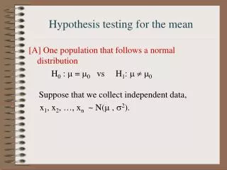
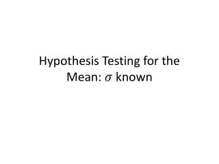
7.3 Hypothesis Testing for the Mean (Small Samples) Statistics Mrs. Spitz Spring 2009
Objectives/Assignment: • How to find critical values in a t-distribution • How to use the t-test to test a mean • How to use technology to find P-values and use them to test a mean . Assignment: pp. 336-339 #1-35 all
Critical values in a t-distribution • In real life, it is often not practical to collect samples sizes of 30 or more. However, if the population has a normal or nearly normal distribution, you can still test the population mean . To do so, you can use the t-sampling distribution with n – 1 degrees of freedom.
Ex. 1: Finding Critical Values for t • Find the critical value to, for a left-tailed test given = 0.05 and n = 21. • Solution: The degrees of freedom are: d.f. = n – 1 = 21 – 1 = 20 To find the critical value, use Table 5 with d.f. = 20 and 0.05 in the “One Tail ” column. Because the test is a left-tailed test, the critical value is negative. So, to = -1.725.
Ex. 2: Finding Critical Values for t • Find the critical value to, for a right-tailed test with = 0.01 and n = 17. • Solution: The degrees of freedom are: d.f. = n – 1 = 17 – 1 = 16 To find the critical value, use Table 5 with d.f. = 16 and = 0.01 in the “One Tail ” column. Because the test is right-tailed, the critical value is positive. So, to = 2.583
Ex. 3: Finding Critical Values for t • Find the critical values, to and –to for a two-tailed test with = 0.05 and n = 26 • Solution: The degrees of freedom are: d.f. = n – 1 = 26 – 1 = 25 To find the critical value, use Table 5 with d.f. = 25 and = 0.05 in the “Two Tail ” column. Because the test is two-tailed, one critical value is negative and one is positive. So, -to = -2.060 and to =2.060
The t-Test for a Mean • To test a claim about a mean using a small sample (n < 30) from a normal or nearly normal distribution, you can use a t-sampling distribution.
Ex. 4: Testing with a Small Sample • A used car dealer says that the mean price of a 1995 Ford F-150 Super Cab is at least $16,500. You suspect this claim is incorrect and find that a random sample of 14 similar vehicles has a mean price of $15,700 and a standard deviation of $1250. Is there enough evidence to reject the dealer’s claim at = 0.05?
SOLUTION: • The claim is “the mean price is at least $16,500.” So, the null and alternative hypotheses are: Ho: ≥ $16,500 (Claim) and Ha : < $16,500 Because the test is a left-tailed test, the level of significance is = 0.05. There are d.f. = 14 – 1 = 13 degrees of freedom and the critical value is to = -1.771. The rejection region is t < -1.771. Using the t-test, the standardized test statistic is:
Solution to 4 continued . . . • The graph shows the location of the rejection region and the standardized test statistic, t. Because t is in the rejection region, you should decide to reject the null hypothesis. There is enough evidence at the 5% level of significance to reject the claim that the mean price of a 1995 Ford F-150 Super Cab is at least $16,500.
Ex. 5: Testing with a Small Sample • An industrial company claims that the mean pH level of the water in a nearby river is 6.8. You randomly select 19 water samples and measure the pH of each. The sample mean and standard deviation are 6.7 and 0.24 respectively. Is there enough evidence to reject the company’s claim at = 0.05? Assume the population is normally distributed.
SOLUTION: • The claim is “the mean pH level is 6.8.” So, the null and alternative hypotheses are: Ho: = 6.8 (Claim) and Ha : 6.8 Because the test is a two-tailed test, the level of significance is = 0.05. There are d.f. = 19 – 1 = 18 degrees of freedom and the critical value is -to = -2.101 and to = 2.101 The rejection regions are t < -2.101 and t > 2.101. Using the t-test, the standardized test statistic is:
Solution to 4 continued . . . • The graph shows the location of the rejection region and the standardized test statistic, t. Because t is not in the rejection region, you should decide not to reject the null hypothesis. There is not enough evidence at the 5% level of significance to reject the claim that the mean pH is 6.8.
Using P-values with t-Tests • Suppose you wanted to find a P-value given t = 1.98, 15 degrees of freedom and a right-tailed test? Using Table 5, you can determine that P falls between = 0.025 and = 0.05, but you cannot determine an exact value for P. In such cases, you can use technology to perform a hypothesis test and find exact P-values.
Ex. 6: Using P-values with a t-Test • The American Automobile Association claims that the mean daily meal cost for a family of four traveling on vacation in California is $124. A random sample of 11 such families has a mean daily cost of $135 with a standard deviation of $20. Is there enough evidence to reject the claim at = 0.05?
Solution: • The TI-83 display below shows how to set up the hypothesis test. The two displays after show the possible results depending on whether you select “CALCULATE” or “DRAW.”
Solution: • The TI-83 display below shows how to set up the hypothesis test. The two displays after show the possible results depending on whether you select “CALCULATE” or “DRAW.” From the displays, you can see that P 0.0981. Because P > 0.05, there is not enough evidence to reject the claim at the 5% level of significance. In other words, you should not reject the null hypothesis.
Study Tip: • Note that the TI-83 display on the far right also displays the standardized test statistic t 1.8241. • 7.3 will be due tomorrow at the end of class. If we don’t finish it up, we will finish on Monday. • 7.4 Monday-Tuesday • 7.5 Wednesday-Thursday • Chapter 7 Review – Friday • Chapter 7 Test – Tuesday on our return. These days could be off one if we don’t finish 7.3 by tomorrow. Keep your homework updated.