Download
1 / 58
580 likes | 651 Views
Modeling Potential Distributions of Species at Large Spatial Extents. Jim Graham Greg Newman, Nick Young, Catherine Jarnevich Natural Resource Ecology Laboratory Oregon State University / Colorado State University. Jim Graham. BS CS and Math from California State University at Chico

E N D
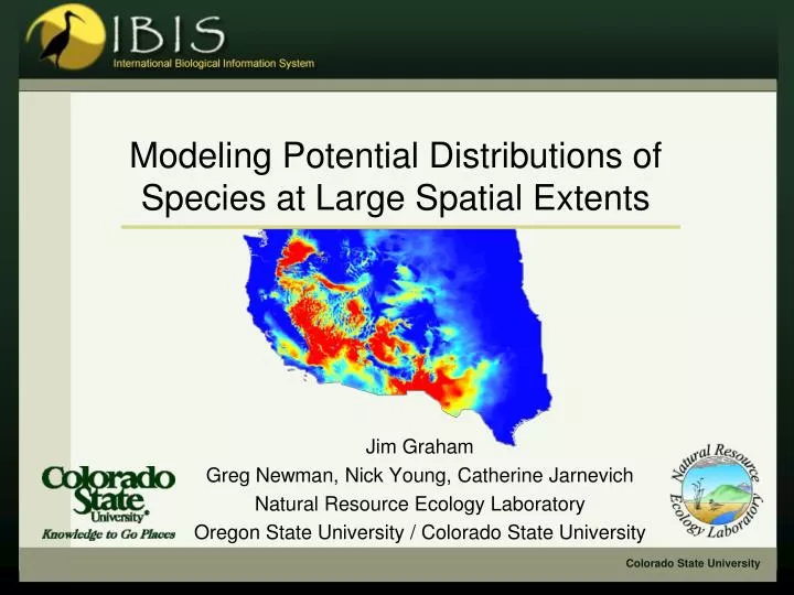
Modeling Potential Distributions of Species at Large Spatial Extents Jim Graham Greg Newman, Nick Young, Catherine Jarnevich Natural Resource Ecology Laboratory Oregon State University / Colorado State University
Jim Graham • BS CS and Math from California State University at Chico • 15 Years Image Processing at HP • 3 Years a CEO for GIS web corp. • PhD in GIS from Colorado State University, Fort Collins • 4 Years as Research Scientist at the Natural Resource Ecology Laboratory • Visiting Professor at OSU
Jim’s Research • Engaging citizen scientists • Web-based GIS • Integrating eco-informatics databases • Global species occurrence databases • Optimal data access for large spatial databases • Habitat suitability modeling at large extents • Risks and impacts of energy production
Invasive Species Mnemiopsisleidyi (comb jelly) Rat attacking New Zealand fantail Photo: David Mudge
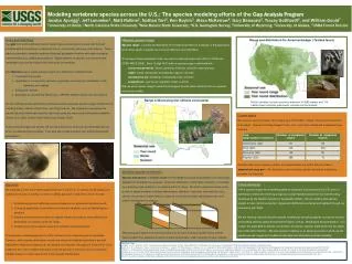
Zebra Mussel Distribution Non-indigenous Aquatic Species Database (USGS), Oct 4th, 2011
Predicting Distributions • Predicting potential species distributions at large spatial and temporal extents • Given: • Limited data • Most have unknown uncertainty • Most biased/not randomly sampled • >90% just “occurrences” or “observations” • Lots of species • Climate change and other scenarios
Occurrences of Polar Bears From The Global Biodiversity Information Facility (www.gbif.org, 2011)
Uncertainty in Data • Experts more accurate in correctly identifying species than volunteers • 88% vs. 72% • Volunteers: 28% false negative identifications and 1% false positive identifications • Experts: 12% false negative identifications and <1% false positive identifications • Conspicuous vs. Inconspicuous • Volunteers correctly identified “easy” species 82% of the time vs. 65% for “difficult” species • 62% of false ids for GB were CB
Tree Sparrow Occurrences House Sparrows Eurasian Tree Sparrows Graham, J., C. Jarnevich, N. Young, G. Newman, T. Stohlgren, How will climate change affect the potential distribution of Eurasian Tree Sparrows (Passer montanus)? Current Zoology, 2011.
100 0 Modeling Process Spreadsheets Occurrences Environmental Layers Temperature Precipitation Modeling Algorithm Model Parameters Habitat Suitability Map Map Generation
Tree Sparrow Model - 2050 Graham, J., C. Jarnevich, N. Young, G. Newman, T. Stohlgren, How will climate change affect the potential distribution of Eurasian Tree Sparrows (Passer montanus)? Current Zoology, 2011
Spatial Modeling Concerns • Over fitting the data • Are we modeling biological/ecological theory? • What does the model look like? • In environmental space vs. geographic space • Absence points? • What do they mean? • Analysis and representation of uncertainty? • Can we really model the potential distribution of a species from a sub-sample?
Two Approaches Occurrence/Presence Mechanistic Occurrences “Greenhouse” experiments Correlate Design Model Model Environmental Layers Generate Generate Map
Geographical Space Observed Occurrences Realized Niche/Distribution Environmental Space Fundamental Niche/Distribution Model Fitted to Occurrences Adapted from Richard Pearson, Center for Biodiversity and Conservation at the American Museum of Natural History
From the Theory of Biogeography + 0 - Salinity Environmental Space Population Growth Niche + 0 - Salinity Temperature Temperature Brown, J.H., Lomolino, M.V. 1998, Biogeography: Second Edition. Sinauer Associates, Sinauer Massachusetts
Germination Percentage Shrestha, A., E. S. Roman, A. G. Thomas, and C. J. Swanton. 1999. Modeling germination and shoot-radicle elongation of Ambrosia artemisiifolia. Weed Science 47:557-562.
Over-fitting The Data? Maxent model for Tamarix in the US: response to temperature when modeled with temperature and precipitation What should the model look like? Maraghni, M., M. Gorai, and M. Neffati. 2010. Seed germination at different temperatures and water stress levels, and seedling emergence from different depths of Ziziphus lotus. South African Journal of Botany 76:453-459.
Maxent Model Parameters • bio12_annual_percip_CONUS, -4.946359908378759, 52.0, 3269.0 • bio1_annual_mean_temp_CONUS, 0.0, -27.0, 255.0 • bio1_annual_mean_temp_CONUS^2, -0.268525818823649, 0.0, 65025.0 • bio12_annual_percip_CONUS*bio1_annual_mean_temp_CONUS, 7.996877654196997, -15579.0, 364506.0 • (681.5<bio12_annual_percip_CONUS), -0.27425992202014554, 0.0, 1.0 • (760.5<bio12_annual_percip_CONUS), -0.0936978541445044, 0.0, 1.0 • (764.5<bio12_annual_percip_CONUS), -0.34195651409710226, 0.0, 1.0 • (663.5<bio12_annual_percip_CONUS), -0.002670474531339423, 0.0, 1.0 • (654.5<bio12_annual_percip_CONUS), -0.06854638847398926, 0.0, 1.0 • (789.5<bio12_annual_percip_CONUS), -0.1911885535421742, 0.0, 1.0 • (415.5<bio12_annual_percip_CONUS), -0.03324755386105751, 0.0, 1.0 • (811.5<bio12_annual_percip_CONUS), -0.5796722427924351, 0.0, 1.0 • (69.5<bio1_annual_mean_temp_CONUS), 0.35186971641045406, 0.0, 1.0 • (433.5<bio12_annual_percip_CONUS), -0.4931182020218725, 0.0, 1.0 • (933.5<bio12_annual_percip_CONUS), -0.6964667980858589, 0.0, 1.0 • (87.5<bio1_annual_mean_temp_CONUS), 0.026976617714580643, 0.0, 1.0 • (41.5<bio1_annual_mean_temp_CONUS), 0.16829480000216024, 0.0, 1.0 • (177.5<bio1_annual_mean_temp_CONUS), -0.10871555671575972, 0.0, 1.0 • (91.5<bio1_annual_mean_temp_CONUS), 0.146912383178006, 0.0, 1.0 • (1034.5<bio12_annual_percip_CONUS), -2.6396398836001156, 0.0, 1.0 • (319.5<bio12_annual_percip_CONUS), -0.061284542503119606, 0.0, 1.0 • (175.5<bio1_annual_mean_temp_CONUS), -0.2618197321200044, 0.0, 1.0 • (233.5<bio1_annual_mean_temp_CONUS), -0.9238257709966757, 0.0, 1.0 • (37.5<bio1_annual_mean_temp_CONUS), 0.3765193693625046, 0.0, 1.0 • (103.5<bio1_annual_mean_temp_CONUS), 0.09930300882047771, 0.0, 1.0 • (301.5<bio12_annual_percip_CONUS), -0.1180307164256701, 0.0, 1.0 • (173.5<bio1_annual_mean_temp_CONUS), -0.10021086459501297, 0.0, 1.0 • (866.5<bio12_annual_percip_CONUS), -0.26959719615289196, 0.0, 1.0 • (180.5<bio1_annual_mean_temp_CONUS), -0.04867293241613234, 0.0, 1.0 • (393.5<bio12_annual_percip_CONUS), -0.11059348100482837, 0.0, 1.0 • (159.5<bio1_annual_mean_temp_CONUS), -0.017616972634255934, 0.0, 1.0 • (36.5<bio1_annual_mean_temp_CONUS), 0.060674971087442194, 0.0, 1.0 • (188.5<bio1_annual_mean_temp_CONUS), -0.03354825843486451, 0.0, 1.0 • (105.5<bio1_annual_mean_temp_CONUS), 0.06125114176950926, 0.0, 1.0 • (153.5<bio1_annual_mean_temp_CONUS), -0.12297221415244217, 0.0, 1.0 • (1001.5<bio12_annual_percip_CONUS), -0.45251593589861716, 0.0, 1.0 • (74.5<bio1_annual_mean_temp_CONUS), 0.026393316564235686, 0.0, 1.0 • (109.5<bio1_annual_mean_temp_CONUS), 0.14526936669793344, 0.0, 1.0 • (105.0<bio12_annual_percip_CONUS), -0.42488171108453276, 0.0, 1.0 • (25.5<bio1_annual_mean_temp_CONUS), 0.003117221628224885, 0.0, 1.0 • (60.5<bio12_annual_percip_CONUS), 0.5069564460069241, 0.0, 1.0 • (231.5<bio12_annual_percip_CONUS), -0.08870602107253492, 0.0, 1.0 • (58.5<bio1_annual_mean_temp_CONUS), -0.23241170568516853, 0.0, 1.0 • (49.5<bio1_annual_mean_temp_CONUS), 0.026096163653731276, 0.0, 1.0 • (845.5<bio12_annual_percip_CONUS), -0.24789751889995176, 0.0, 1.0 • 'bio1_annual_mean_temp_CONUS, -6.9884695411343865, 232.5, 255.0 • (320.5<bio12_annual_percip_CONUS), -0.10845844949785532, 0.0, 1.0 • (121.5<bio1_annual_mean_temp_CONUS), -0.12078290084760739, 0.0, 1.0 • (643.5<bio12_annual_percip_CONUS), -0.18583722923085083, 0.0, 1.0 • (232.5<bio1_annual_mean_temp_CONUS), -0.49532279859757916, 0.0, 1.0 • (77.5<bio12_annual_percip_CONUS), 0.09971599046855084, 0.0, 1.0 • (130.5<bio1_annual_mean_temp_CONUS), -0.01184619743061956, 0.0, 1.0 • (981.5<bio12_annual_percip_CONUS), -0.29393286794072015, 0.0, 1.0 • `bio12_annual_percip_CONUS, 0.023135559662549977, 52.0, 147.5 • 'bio1_annual_mean_temp_CONUS, 1.0069995641400011, 216.5, 255.0 • `bio1_annual_mean_temp_CONUS, 0.9362466512437257, -27.0, 16.5 • (397.5<bio12_annual_percip_CONUS), -0.02296169875555788, 0.0, 1.0 • `bio12_annual_percip_CONUS, 0.14294702222037983, 52.0, 251.5 • (174.5<bio1_annual_mean_temp_CONUS), -0.01232159395283821, 0.0, 1.0 • 'bio1_annual_mean_temp_CONUS, -1.011329703865716, 150.5, 255.0 • `bio12_annual_percip_CONUS, 0.12595056977305263, 52.0, 326.5 • 'bio1_annual_mean_temp_CONUS, -0.6476124017711095, 119.5, 255.0 • 'bio1_annual_mean_temp_CONUS, 1.737841121141096, 219.5, 255.0 • (90.5<bio1_annual_mean_temp_CONUS), 0.012061755141948361, 0.0, 1.0 • `bio12_annual_percip_CONUS, 0.1002190195916142, 52.0, 329.5 • `bio12_annual_percip_CONUS, 0.3321425790853447, 52.0, 146.5 • `bio12_annual_percip_CONUS, -0.3041756531549861, 52.0, 59.0 • (385.5<bio12_annual_percip_CONUS), -0.0014858371668052357, 0.0, 1.0 • (645.5<bio12_annual_percip_CONUS), -0.02553082983087001, 0.0, 1.0 • 'bio12_annual_percip_CONUS, -4.091264412509243, 532.5, 3269.0 • `bio1_annual_mean_temp_CONUS, -0.35523981011398936, -27.0, 111.5 • `bio1_annual_mean_temp_CONUS, -0.21070138315106224, -27.0, 112.5 • `bio1_annual_mean_temp_CONUS, 0.22680342516229093, -27.0, 18.5 • (13.5<bio1_annual_mean_temp_CONUS), -0.04258692136695379, 0.0, 1.0 • `bio1_annual_mean_temp_CONUS, 0.12827234634968193, -27.0, 19.5 • linearPredictorNormalizer, 2.2050375426546283 • densityNormalizer, 1311.2581836276431 • numBackgroundPoints, 10000 • entropy, 8.358957722359722 162 Parameters Maxent model from Tamarix model of western US using precipitation and temperature.
Geographical Space Observed Occurrences Realized Niche/Distribution Environmental Space Fundamental Niche/Distribution Model Fitted to Occurrences Adapted from Richard Pearson, Center for Biodiversity and Conservation at the American Museum of Natural History
United States Environmental Space Tamarisk Occurrences
Can we? • Create a species distribution modeling method that: • More closely matches ecological theory? • Allows visualization of the model in environmental space? • Does not use absence points? • Allows integration of physiological knowledge and occurrence data? • Allows editing the model to try scenarios? • Represents uncertainty?
Some Caveats • We are modeling “observations” • Modeling occurrences with some uncertainty • Modeling the realized niche if the data is a complete sample for the environmental space the species currently occupies • Modeling the fundamental niche if B is true and the species is covering it’s full possible range of habitats • Habitat Suitability Modeling • Predicting the potential species distribution
Problems with Polynomials f(x) = a0 + a1x + a2x2 + ... + anxn , where an ≠ 0 and n ≥ 2 • Lack flexibility • Not well behaved at boundaries Wikipedia.com
Bezier and Spline Curves P1 P0 P2 P3 Wikiepedia.com
International Biological Information Science Modified Bezier Curves S3 S2 P2 P3 S1 P0 P1 S0
International Biological Information Science HEMI Tamarix Model 107 AUC: 0.76 Min Temp of coldest Month (°C*10) Potential Habitat 5 Points -> 10 Parameters -231 Unsuitable Habitat 46 3385 Annual Precipitation (mm)
Area Under the Curve Metric • Area Under the Curve (AUC) • 1=Perfect • 0=Worthless
International Biological Information Science Potential Habitat Potential Habitat Unsuitable Habitat
International Biological Information Science Global Tamarisk Map? 1.0 Habitat Suitability 2.0
Migration Animations • Jim’s web site • http://tinyurl.com/6krghts • Gray whale model • http://tinyurl.com/4xtmzho • Barn swallows
Conclusions • We can visualize models in environmental space • At least in 2 dimensions • We can build constrained models and edit the models for scenarios • We can reduce the complexity of the models • Absence points are not required • Categorical variables have to be modeled separately for each category
Next Steps • Characterize a number of species to determine how to constrain the envelopes • Develop likelihood model to fit Bezier curves? • Include uncertainty analysis and error surfaces • Move HEMI to the web? • More “good” data!
Acknowledgements • Tom Stohlgren, Lane Carter, Abby Flory, Paul Evangelista, Sunil Kumar, Alycia Crall, Kirstin Holfelder, Sara Simonson, Lee Casuto, Annie Simpson, Jeff Morisette, and many more… • Funding: USGS, NASA, NSF, GBIF, NBII • NSF Grant #OCI-0636210
Deep Water: DOE • Risks and Impacts of Exploration and Production of Fossil Fuels: • Initially in Gulf of Mexico • Expanding to the Arctic • Scope: • Sub-surface, flow modeling, environmental impacts, economic and social impacts • Department of Energy Funding • http://www.netl.doe.gov/careers/fellowships.html
US IS Databases • National: NIISS, EDDMaps, iMapInvasives, Discover Life, SERC, NAS NWIPC GLIFWIC IPANE ICE SWEMP Texas Invaders SEEPPC
International Biological Information Science • Mapping Species Distributions: Spatial Inference and Prediction (Ecology, Biodiversity and Conservation)
International Biological Information Science Two Approaches • Mechanistic/Greenhouse: • Limited genotypic variation • Limited ecosystem complexity • Widely used in agriculture • Occurrence/Presence Based • Do the models match ecological theory? • Widely used with non-agricultural species • Invasive species, T&E • Even humans
Environmental Space: Earth 2010 Maximum Mean Annual Temperature (C * 10) Number of Samples Minimum Annual Precipitation
System Architecture Client Internet Server Database Job Controller Web Server Browser Jobs HTML Pages PHP Pages Spatial Library Raster Layers Images Images Clients Web Services
International Biological Information Science Impacts • Shift management areas • Agriculture/Aquaculture • Wildlife reserves • Natural areas • Migration corridors • Shift priorities • Invasive species • Threatened and endangered species • Help make decisions for better management
Data Issues • All data has uncertainty • Need to quantify and maintain uncertainty • From field through to distribution maps! • Don’t need every occurrence: • Need environmental range covered • Need to understand barriers to dispersal
Absence Points • What do they mean? • We did not find the species there at some point in time • Was it there before? • Was it removed? • Has it been able to get there? • We should plant it and see what happens! • Pseudo-random points?
Database Who & When Organizations Where What Projects Taxon Units Organism To Area Area (Name, Code) Visit (Date) Organism Data (TSN) Spatial Data (X, Y) Treatments Attributes Pathways?