Download
1 / 23
230 likes | 390 Views
Turbulent dynamics of pipe flows captured in a ‘2 +ɛ’-dimensional model. Ashley P. Willis LadHyX, École Polytechnique, Palaiseau, France., Rich Kerswell Dept. of Maths., University of Bristol, U.K. + Yohann Duguet, Chris Pringle. θ. z. r. Distinct spatial structures:.

E N D
Turbulent dynamics of pipe flows captured in a ‘2+ɛ’-dimensional model Ashley P. Willis LadHyX, École Polytechnique, Palaiseau, France., Rich Kerswell Dept. of Maths., University of Bristol, U.K. + Yohann Duguet, Chris Pringle
θ z r Distinct spatial structures: Localised “puff” plot of axial vorticity Re >~ 1650 Expanding “slug” Re >~ 2250 Pipe flow Parabolic laminar flow D, diameter U, mean axial flow (constant) Re = UD / ν No linear instability
Temporal characteristics Peixinho & Mullin (2006), PRL Energy t sudden relaminarisation
Re~ 750 Repuff-slug~2250 Disturbance amplitude exact travelling waves F&E (2003) W&K (2004) (all unstable) Issues : Does turbulence become sustained? How are TWs related to turbulence? How does localised turbulence remain localised!? Re
θ z r Aim: Want to study pipe flow as a subcritical dynamical system. Problems: System has a vast number of degrees of freedom! Short periodic pipes cannot capture the spatio-temporal characteristics. Full 3-dim calculations are expensive. Parabolic laminar flow D, diameter U, mean axial flow (constant) Re = UD / ν Localised “puff” plot of axial vorticity Expanding “slug” Q: Can we reduce the system but capture localised structures?
localised in z → keep axial resolution • near-wall structures important, detachment from wall during relaminarisation; r → keep radial resolution 1 1 • → leaves only θ . Minimal 3-dimensionalisation: Fourier modes, m = −m0, 0, m0 only. • i.e. only 3 degrees of freedom in θ : • a mean mode, • a sinusoidal variation in θ, • an azimuthal shift of the sinusoid. ‘ɛ’ ‘2+ɛ’-dimensional model.
Do we capture the spatial characteristics? puff → slow delocalisation → slug ‘2+ɛ’-dim. 160,000 d.f. (Lz = 50 diameters, 25 shown) Re = 2600, 3200, 4000 3-dim. 3,600,000 d.f. Re = 2000, 2300, 2700
Reduced model preserves temporal characteristics... long-term transients, sudden decay, memoryless (Lz = 50 diameters, Re=2800)
τ ~ 1/(Rec-Re)5 Rec = 3450
Disturbance amplitude exact travelling waves Lower branch associated with `edge’ Re
Amplitude Turbulent ‘Edge’ TW Laminar t
The laminar-turbulent ‘edge’(short pipe Lz = π diameters; 10,000 d.f.)
Model has exact TW solutions (Newton-Krylov code by Yohann Duguet) fast axial flow slow axial flow
The laminar-turbulent ‘edge’(short pipe Lz = π diameters; 10,000 d.f.)
Roll + wave energy Amplitude ~ Re-3/2
The ‘edge’ in a long pipe (work in progress) Turbulence at increasing Re Re = 2600, 3200, 4000 Edge at high flow rate, Re = 4000 exact soln. (Chris Pringle) exact soln. (Yohann Duguet)
Edge at high flow rate, Re = 4000 Re = 10000 see Yohann’s talk
Model has TWs, long-term transients, memoryless, spatially localised puffs, slugs, chaotic edge state. • Amplitude of rolls+waves ~ Re-3/2 . • Can we use the model to explain why puffs stay localised? • Is there a measure that predicts the puff-slug transition? • ..or a sensitive measure that pre-empts relaminarisation? • What is the effect of ‘noise’ on transitions, relam., puff-slug...? • What is the ‘minimal flow unit’ that produces transients? • Are there exact localised solutions on the edge? periodic orbits? Ref.: arXiv.org:0712.2739
Time-averaged profiles within the puff Full 3-dim, Re = 2000 2+ɛ-dim model, Re = 3000