Download

1 / 123
1.27k likes | 1.74k Views
Models of Yield Curve and Yield Curve Dynamics. Outline. We are going to focus on just on a few of the models: Random walk model of interest rates Mean – reverting interest rates The Cox – Ingersoll – Ross Model The BDT Model. Binomial Model of Bond Prices.

E N D
Outline • We are going to focus on just on a few of the models: • Random walk model of interest rates • Mean – reverting interest rates • The Cox – Ingersoll – Ross Model • The BDT Model
Binomial Model of Bond Prices • It is tempting – and commonly done – to extrapolate the binomial stock price model to bond prices. This can create some problems, because it ignores certain aspects of bond prices, namely: • Bonds are not infinite lived • Bonds must converge to par (100) at their maturity • Bonds can go to 0
u2 P uP ud P P dP d2 P • If we work with a typical Cox, Ross, Rubinstein model: Where u = e σ ((T-t)/N)1/2 = e σ (dt)1/2 = 1/d and the up – jump probability is: q = 0.5 + 0.5 u/σ (dt)1/2 This results in bond price has a distribution dP/P= u dt + d2 which means that bond prices are lognormally distributed, even at maturity. • As a result, the CRR type of model is not widely used
u2 r (t) ur (t) R (t) rd r (t) dr (t) d2 r (t) Binomial Model of Interest Rates • Another approach, of course, would be to simply model the underlying interest rate as a binomial model. This, in fact, is one of the basic techniques used in term structure modeling today.
1 bu (1,2) b (0,2) 1 bd (1,2) 1 Binomial Model of Interest Rates • Let q be the probability of an up jump and (1-q) the probability of a down jump • In reality you would like for the probability to adjust depending on the level of rates, but for starters we will ignore that possibility. • Consider how a two discount bond will evolve:
Binomial Model of Interest Rates • We now invoke the notion of the local expectations Hypothesis. • This says, essentially, that the expected return over one period on any (default free) bond should be the same as the one-period rate prevailing at that time. • Under LEH, therefore, at time t=1, this must hold: • 1 / bu (1,2) = 1 + ur (t) and 1 / bd (1,2) = 1 + dr (t) • Recall that ur(t) and dr(t) are rates, not products necessarily
q.1 + (1-q) 1 q.1 + (1-q) 1 1 1 bu (1,2) = bd (1,2) = = = 1 + ur (t) 1 + ur (t) 1 + ur (t) 1 + ur (t) Binomial Model of Interest Rates • We can rearrange these to get a pricing method: • We can now work backwards to get a price at time 0
= (1 + r(t)) b (0,2) q . bu (1,2) + (1-q) bd (1,2) B (0,2) = 1 + r(t) Binomial Model of Interest Rates • We begin with the LEH condition: • This is really nothing more than a variant of how we have been pricing options all along • This whole business of the LEH is really just to justify the following: if you are at a node in lattice where the rate is r, then all bonds should be discounted at that rate q . bu (1,2) + (1-q) bd (1,2) or
19.531 15.625 12.50 12.5 10.00 10.00 8.00 8.00 6.40 5.12 Example 17 - 1 • The initial one-period rate is 10%, the up factor (u) is 1.25 and d=0.80. We define the probability of an up (or down) move as 0.50. Based on this, rates evolve as:
1 12.50% 0 10% 1 8% Binomial Model of Interest Rates • Given this structure we can really start to calculate some interesting values • What is a one-period zero-coupon bond worth? • To answer this we can examine just the first two levels of the lattice. The bond pays $1 with certainty at the end of the period Now the first thing to notice is that the only relevant rate is the one at the central node, since it is the correct discount rate for the time period 0-1. In essence r 1,1=12.5 and r 1,0 = 8.0 become effective at the start of period 1, while the $1 cash flows at paid at the end of period 0.
$1 12% 10 % 8% $1 Binomial Model of Interest Rates • Within the lattice we tend to draw the end of 0 and the beginning of 1 as occurring at the same point, but they are actually different. In fact, some people draw these as:
0.5($1) + 0.5($1) 1 + r 0,0 $1(0.5) + $1(0.5) 1,2 = b 1,1 = 1,2 1.12 b 12% 0,2 1,1 $1(0.5) + $1(0.5) 1,2 = b b 1,0 = 0,0 1,2 b 8% 1,0 Binomial Model of Interest Rates • So to get the 1 period bond price you do the following: • We can easily extend this to a two period example $1/1.10 b (0,1) = = = 0.9091 $ 1 0.8889 $ 1 0.9259 1.08 1(0.88) + 1(0.92) 0,2 = b 0,0 = 0.8249 1.10 $ 1
$1 0.889 12% 0,2 b 0.8249 $1 0,0 0.9259 8% $1 Binomial Model of Interest Rates • So the overall lattice looks like: • Frankly the superscript is frequently suppressed – people assume you know which bond you are using. • Notice that we now know the price of a zero coupon bond for periods 1 and 2, i.e 90.91 and 82.49.
0,1 1 1 Price0 = = 0.9091 = b 0,0 (1+y1) (1+y1) 0,2 1 = 0.8249 = b 0,0 (1/0.8249)1/2 – 1 = y2 (1+y2)2 Y2 = 10.10% Binomial Model of Interest Rates • From this we can determine the yields for one and two period zero coupon bonds: 1/0.9091 – 1 = y1 y1 = 10%
1 0.8889 0.8249 1 0.9259 1 Binomial Model of Interest Rates • We can now show the evolution of the two period bond prices • We can now apply the same basic methodology to a three period bond
1 0.8649 15.625% 0.7884 1 12% 0.7475 0.9091 10% 10% 1 0.8560 8% 0.9398 6.4% 1 Binomial Model of Interest Rates
$1(0.5) + $1 (0.5) $1(0.5) + $1 (0.5) $1(0.5) + $1 (0.5) 2,3 2,3 2,3 = = = = = = 0.9091 0.9398 0.8649 1,3 0,3 2,3 0.5(0.7884) + 0.5(0.8560) 0.5(0.9091) + 0.5(0.9398) 0.5(0.8649) + 0.5(0.9091) b 2,0 b 2,2 b 2,1 b 1,1 b 1,0 b 0,0 = = = = = = 0.7884 0.7475 0.8560 1.156 1.064 1.10 1.12 1.08 1.10 Binomial Model of Interest Rates Notice a few things here. First, we can solve for the three period yield : Y3 = (1/0.7475)1/3 – 1 = 10.1888% Y1 =10% Y2 = 10.10% Y3 = 10.188% Thus we now know the three period zero coupon yield curve :
0.7884 0.8249 0.8560 Binomial Model of Interest Rates • We can also talk about the evolution of the two-period zero coupon yield over time. We know that at time 0 the two period zero coupon bond was worth 0.8249, and has a yield of 10.10%. • Based on our results we know that a two year bond at node (1,0) is worth 0.8560 and a two year bond at node (1,1) is worth 0.7884. • From this we got the evolution of two year, constant maturity bond prices
12.622 10.10 0.080844 t = 0 t = 1 Binomial Model of Interest Rates • Now the two-year zero coupon rate at node 1,0 is given by: y (2)1,0 = (1/0.8560)1/2 – 1 = 0.80844 • And at 1,1: y (2)1,1 = (1/0.8560)1/2 – 1 = 0.80844 • So the two year constant maturity zero coupon yield evolves as:
y12 = 0.125 y22=0.12662 y1 = 0.10 y2=0.1010 y1 = 0.080 y2 =0.080844 Binomial Model of Interest Rates • Thus you can see that the two year constant-maturity rate evolves, just as the one period rate evolves • The yield curve is, therefore, evolving over time, but the only factor driving this yield curve is the evolution at the one period interest rate. Notice that the yield curve is not moving in parallel, however. It is steeper at node 1,1 than at 0,0 and it is flatter at 1,0 then at 0,0
Binomial Model of Interest Rates • If we extend our model out more periods we can observe the evolution if more distant points on the yield curve – for example we could see how the three year constant maturity rate evolved. • In fact, if we wanted to we could describe the evolution of the entire yield curve as being driven by this single factor. • Note that you have to pay attention to some issues here. You can discuss (as the book largely does) how a single bond evolves its price through time. For example you could see how a 4 period zero coupon starts at a given price and then in period 1 has a new price (or set of prices) and then get another set of prices in times 2 & 3.
Binomial Model of Interest Rates • But you are observing a 4 year bond in time 0, a 3 year bond in time 1, etc. You also want to pay attention to how the four year (or 3 year, etc) rate varies from period to period and from node to node. To do that you have to look at different bonds through time. • I can also extract implied forward rates and see how they evolve over time, based on how the yield curve evolves – which again is based on the evolution of the one period “spot” rate (i.e. one period yield). • To see this, let’s return to our lattice describing how the yield curve evolves over the first two periods:
y1=15.625% y12 = 0.125 y22=0.12662 y1 = 0.10 y2=0.1010 y1=10% y1 = 0.080 y2 =0.080844 y1=6.4% Binomial Model of Interest Rates • Recall that the forward rate is the rate to which you can contract today to borrow in a future period. So at any point the one period forward rate is given by: • f(1,2) = ((1+y2)2 / (1+y)) – 1 • So at node 0,0: f(1,2)0,0 = ((1.1010)2 / (1.10)) – 1=10.2% • Note that this is not the expected spot rate in one period
12.824 10.20 8.1688 Binomial Model of Interest Rates • At node 1,0 that forward rate is given by: • f(2,3)1,0 = ((1.080844)2 / (1.08)) – 1=8.1688 • And at node 1,1 it is given by: • f(2,3)1,1 = ((1.12662)2 / (1.125)) – 1=12.824 • So we get an evolution of the one period forward curve as So the one period spot rate evolution drives not only the yield curve evolution, but also the evolution of the forward rate. In fact the forward rate and spot rates roles are sometimes reversed. In the HJM model it is the forward rate which is allowed to evolve and the spot rate evolution is implied by that evolution.
Binomial Model of Interest Rates • Now there are a couple of points we can make here about using this lattice structure. It is very good for pricing options, interest rates and other contingent claims, and you discount everything at the one period rate. • Let’s look at a couple of examples
1 0.8649 15.625% 1 12.5% 10% 0.9091 10% 1 8.0 % 0.9398 6.4% 1 Basic Bond Option • Let’s say that you hold a call option which gives you the right, at the beginning of period 3 (so the option expires at the end of period 2) to purchase a one period bond at price 90. What is this option worth today? • Let’s begin by recalling what our evolution of rates and prices looks like:
Basic Bond Option • So at nodes (2,0), (2,1), and (2,2) we get one period zero coupon bond prices of 0.9398, 0.9091 and 0.8649 respectively. Since our strike is 0.90, our payoffs to the option are given by: • C2,0 = max (0, 0.9398 – 0.90) = 0.0398 • C2,1 = max (0, 0.9091 – 0.90) = 0.0091 • C2,2 = max (0, 0.8649 – 0.90) = 0 • We can now move backwards through the lattice to determine the price of the option C 2,2=0 C 1,1 =0.0040 0.125 C 0,0 0.10 C 2,1 =0.0091 C 1,0 =0.0226 0.08 C 2,0 =0.0398
0.5(0.02263) + 0.5 (0.004) 0.5(0.0091) + 0.5 (0) 0.5(0.0091) + 0.5 (0.0398) = = = = = = 0.0121 0.2263 0.0040 C 0,0 C 1,1 C 1,0 1.125 1.10 1.08 Basic Bond Option Or 1.212 on a $100 bond
Interest Rate Cap • Let’s say that you are a bank. Your average depositor puts money into 2 year CDs. • So you have significant exposure to the two year zero coupon bond rate (realize that in any year ½ of your depositors roll into new CDs at the rate for that year). • Since you wish to manage your exposure you elect to use an interest rate cap on the two year zero coupon bond rate. • Let’s say that we have $100 million in total deposits, so you hedge $100 million notional. Your payoff is equal to two years interest on the notional amount.
y1=15.625% y2=15.7706% y12 = 0.125 y22=0.12662 y1 = 0.10 y2=0.1010 y1=10% y2=10.10% y1 = 0.080 y2 =0.080844 y1=6.4% y2=6.471% Interest Rate Cap • Recall that today the two year zero coupon bond rate is 10.10%, and let’s assume that this is the strike rate. The payoff to the cap would be: • Cap t = [ $100 . Max (0, zero 2,t – cap-rate)] • Recall earlier that we noted that the yield curve was evolving according to:
0.5(0.8366) + 0.5 (0.8888) 0.5(0.9259) + 0.5 (0.95129) 0.5(0.8888) + 0.5 (0.9259) = = = = = = 0.74611 0.82486 0.88213 P(2) 2,1 P(2) 2,2 P(2) 2,0 1.10 1.15625 1.064 Interest Rate Cap • I have extended this another period using the rates found on page 601. • P(1)3,3 = 1/1.19531 = 0.8366 • P(1)3,2 = 1/1.125 = 0.8888 • P(1)2,1 = 1/1.108 = 0.9259 • P(1)2,0 = 1/1.10512 = 0.95129 y(2)2,2=((1/0.7461)1/2) -1=15.7706% y(2)2,1=((1/0.82486)1/2) -1=10.10% y(2)2,0=((1/0.88213)1/2) -1=6.471%
Cf2,2=5.67=V 2,2 y1=0.15625 y2=0.157706 V1,1=5.08 Cf=2.56 y1=0.125 y2=0.12662 V0,0=2.039m Cf0,0=0 y1=0.10 y2=0.1010 Cf2,1=0=V 2,1 y1=0.100 y2=0.1010 V1,0=0 Cf1,0=0 y1=0.08 y2=0.08084 Cf2,0=0=V 2,0 y1=0.064 y2=0.06471 Interest Rate Cap • So I can now convert this into cash flows. Recall that the cap pays off annually based on the $100 million notional. I am simplifying by assuming the cap pays immediately. It normally would not.
0.5(5.08) + 0.5 (0) 0.5(CF 2,2) + 0.5 (CF 2,1) 0.5(5.67) + 0.5 (0) 0.5(CF 1,1) + 0.5 (CF ,1,0) = = + + CF 1,1 CF 0,0 V 0,0 V 1,1 = = + 0 = 2.309m + 2.56 = 5.08m 1.125 1.10 1 + y1 1 + y1 Interest Rate Cap • CF 2,2 = 100 . Max(0,y2 – cap-rate) = 100 . Max(0, 0.157706-0.1010) = 100m X 0.0567 = 5.67 million • CF 2,1 = 0 • CF 2,0 = 0 • CF 1,1 = 100 . Max(0, 0.12662-0.1010) = 2.562 m • CF 0, 0 = 0
110 Call = 10 F = 10 100 90.91 Call = 0 F = -9.09 Interest Rate Cap • Let’s say that the initial futures price is 100, and it can raise or fall by 10%, farther, the risk fee rate is 5%, and the strike is 100. • Assume we construct a portfolio consisting of : • 1 short call • futures contracts
110 -10 + 0.5238(10) = -4.762 100 90.91 0 - 0.5238(9.09) = -4.762 Interest Rate Cap • And we select such that the portfolio has the same value in all states of the world at time 4: • - 10 + 10 = -9.09 19.09 = 10 = 10/19.09 = 5.238 • Thus the portfolio value is: Thus the portfolio will be worth –4.762/1.05 = -4.534 today The time 0 futures contract is worth 0, so the portfolio value is given by: -4.534 = 0 –(1)4.534 So the call value is 4.534
Interest Rate Cap • We can generalize this : • = (Cu – Cd) / (Hu – Hd) = Cu – Cd / (u- d) H • The value at the end of the time period, the is always: • (Hu – H) - Cu Since this is by construction the top part if the lattice / you could do this with the bottom as well) • Which has present value: • [(Hu – H) - Cu] e –rT • And we know that the value of the futures contract today must be zero, so the portfolio value at time 0 only comes from the time 0 option value: • - c = [(Hu – H) - Cu] e –rT
or c = e –rT 1-d 1- d [ Cu + ( 1- ) Cd ] u - d u – d c = e –rT [ P Cu + (1-P) Cd] Where P = (1-d)/(u-d) Interest Rate Cap • Substituting for and simplifying will result in: • Note: It may be optimal to exercise an American call on a bond futures contract early, although it generally is not optimal to do so on a call on the bond itself • To see this let’s consider the following:
p(ult – k) + (1-p)(dh – k) C = max [ H – k, ] 1 + r (1-d)/(u-d)(uk – k) + (1- (1-d)/(u-d) )(dh – k) C = max [ H – k, ] 1 + r Interest Rate Cap • Assume that the call will be in the money regardless of the final state, i.e. both Cu and Cd > 0. So Cu = Hu – k and Cd = Hd – k. • Consider the time 0 price for the option: • Substitute (1-d)/(u-d) for p: C = max [ H – k, (h – k)/(1+r)], so early exercise is indeed optimal
Properties of Rates • Now, so far, we have ignored the question of how we develop the interest rate lattice. • Clearly we want to build it in a way that is consistent with basic interest rate processes that we have observed over time. • Before we can begin with a specific lattice model, therefore, we want to fully understand what we want in an interest rate model. • We want the interest rate model to be stochastic. • We want the model to exhibit mean-reversion. • Why? Because in reality rate exhibit this property!
A Simple Model with Mean Reversion • Sundaresan presents a simple model that incorporates mean reversion. • This model is not really that great for pricing assets, but it is good for illustrating a few properties of mean reversion. • The model works as follows. • The one-period interest rate is assumed to be bound by an upper limit of 2μand a lower limit of 0. • Over one step in the binomial lattice, rates can rise of fall by an amount δ, which is selected based on the time-step of the lattice. • The probability of an up-jump from a given node in the lattice (t,j), is given by: • This generates a model that looks like this:
A Simple Model with Mean Reversion Upper limit: r=2μ Lower limit: r=0
A Simple Model with Mean Reversion • Notice that for any node (t,j), the rate can be represented as: rt,j = r0,0+j*δ-(t-j)δ • Thus, r1,1 = r0,0 + (1) δ-(1-1) δ = r00+ δ • Similarly, r3,2 = r0,0+(2) δ-(3-2) δ = r0,0+2 δ-1 δ = r0,0+ δ • And r3,0=r0,0 + (0) δ – (3-0) δ = r0,0-3 δ • Example: • Assume r0,0=10%, δ=1%, and μ=12%. What would the lattice and the transition probabilities look like?
A Simple Model with Mean Reversion Upper limit: r=2μ=2(12%)=24% Lower limit: r=0
A Simple Model with Mean Reversion • Notice that as the lattice grows toward 2μ or 0, that the probabilities force you to move back to the center of the lattice. • At the two boundaries, you get the following probabilities of up and down jumps: • If r=2μ, then q=0, so (1-q)=1, meaning that a “down” jump is guaranteed. • If r=0, then q=1, and (1-q)=0, meaning that an “up” jump is guaranteed. • You can then price bonds, options, swaps, etc. backwards through the lattice as we did earlier in the model.
More Advanced Models • Now, one has to be a little bit careful when talking about term structure models as to what is being meant. • Sometimes people refer to a specific incarnation of a lattice as being the “model”. What they mean is both the underlying distribution of interest rates and the numerical method (the lattice) that insures they price bonds using that distribution. • In other contexts people are referring only to the underlying distribution of rates. • This is really the more general way of thinking of the term structure model, since there may be more than one numerical procedure that can determine prices under that distribution. • We are going to first examine a model known as the Vasicek model and one of its variants known as the Cox, Ingersoll, and Ross (CIR) model.
More Advanced Models • Theorists really like the Vasicek and CIR models because they are General Equilibrium models. • This means that they are consistent within an entire economy that is defined by just a few parameters. • They are also well-liked because you can get closed-formed solutions for zero coupon bonds. • The difficulty with these models is that they are notoriously difficult to calibrate. • This means that the input parameters they require are very difficult to estimate econometrically to within the level of accuracy needed for pricing real-world assets. • There are many numerical models that people use that are consistent with Vasicek and CIR, but we will primarily focus on their use within Monte Carlo.
Vasicek Model • The Vasicek class of models assume that only one fact, the one-period interest rate (r), determines the entire term structure. The process that r follow is: (note this differs from Sundaresan) where: • r = the spot rate • γ = a speed of adjustment factor • μ = the long-run mean of the interest rate process • σ = the volatility of the short-run rate • dz = a white noise process.
Vasicek Model • The model admits closed form solutions for a zero coupon bond: