Download
1 / 20
210 likes | 430 Views
Describing Quantitative Data Numerically. Symmetric Distributions Mean, Variance, and Standard Deviation. Symmetric Distributions. Describing a “typical” value for a set of data when the distribution is at least approximately symmetric allows us to choose our measure of center:

E N D
Describing Quantitative Data Numerically Symmetric Distributions Mean, Variance, and Standard Deviation
Symmetric Distributions • Describing a “typical” value for a set of data when the distribution is at least approximately symmetric allows us to choose our measure of center: • We can use either • Mean • Median
Finding the Mean of a Distribution • The mean of a set of numbers is the arithmetic average. We find this value by adding together each value and then dividing by the number of values we added together • The formula for the mean is:
Let’s see the Formula in Action • Consider Babe Ruth’s HR data • A check of a dotplot indicates that the distribution is approximately symmetric
So… the first step is to add all the values 54 + 59 + 35 + 41 + 46 + 25 + 47 + 60 + 54 + 46 + 49 + 46 + 41 + 34 + 22 = 659 • Now we need to divide that sum by the number of values we added together.
So the mean of the data is 43.9333. Now, if we wish to talk about the “typical” number of home runs for Babe Ruth (and we ALWAYS wish to talk about the context of our data!), we could say something like… On average, Babe Ruth hit approximately 44 home runs per season during the 15 seasons he played.
Remember that although the center is a very important part of our description, we also need to look at the spread of the distribution. • When we use the mean as our measure of center, we use the standard deviation as our measure of spread. • We can think of standard deviation as “an average distance of values from the mean” • To calculate the standard deviation by hand, we’ll make a data table…
Creating the Data Table • The first part of our formula indicates that we need to find the distance from the mean for each of our values (x – x)
Now that we know the individual distances for each value, we want to find an “average” of those distances. • To find an average we have to add all the values together • We find, though, that the sum of those values is always zero. • Why? Because some of the values are above the mean (positive values) and some are below (negative). The positives and negatives cancel each other out. • So what values can we use to find the “average” distance from the mean for a set of values?
One way to get rid of the negative values in these distances is to square each of the values. That’s exactly what our formula tells us to do. (x – x)2 • Once we have these values, to find the average we must add them together
The final step in finding an average is to divide by the number of values we added together, but our formula is a little different here. • Instead of dividing by the total number of values we added together, we divide by 1 less than the total. • Why? We have taken a “sample” of the data instead of every piece of data in the population. Since another “sample” would produce a slightly different mean, it would also produce a slightly different standard deviation. Dividing by 1 less than the total number of values added together will give us a slightly larger spread to account for this sampling variation.
So, we divide the “sum of the squared deviations” by n-1 • We have now calculated everything inside the square root sign • This value is an important one—It is called the Variance --S2
Since the units of the variance are not the same as our original units, we have one more calculation we must make. • The square root of the variance will restore the original units and give us the “average distance from the mean”—the standard deviation • S = 11.2470
TI-TipsMean, Variance, & Standard Deviation Find the MEAN • Enter the data into a list • 2nd STAT • MATH • 3:mean(list name) • If you have used a frequency list, 3:mean(data list, freq list)
TI-Tips Find the Variance • Enter the data in a list • 2nd STAT • MATH • 8:variance(list name) • If you have used a frequency list, 8:variance(data list, freq list)
TI-Tips Find Standard Deviation • Enter the data in a list • 2nd STAT • Math • 7:stdDev(list name) • If you have used a frequency list, 7:stdDev(data list, freq list)
Additional Resources • Practice of Statistics: Pg 30-34, 43-46 • Homework: HW 1.2: 1a-d