Download
1 / 36
360 likes | 439 Views
Section 1.3 Describing Quantitative Data with Numbers. Mrs. Daniel AP Statistics. Section 1.3 Describing Quantitative Data with Numbers. After this section, you should be able to… MEASURE center with the mean and median MEASURE spread with standard deviation and interquartile range

E N D
Section 1.3 Describing Quantitative Data with Numbers Mrs. Daniel AP Statistics
Section 1.3Describing Quantitative Data with Numbers After this section, you should be able to… • MEASURE center with the mean and median • MEASURE spread with standard deviation and interquartile range • IDENTIFY outliers • CONSTRUCT a boxplot using the five-number summary • CALCULATE numerical summaries with technology
Measuring Center: The Mean To find the mean (pronounced “x-bar”) of a set of observations, add their values and divide by the number of observations. If the n observations are x1, x2, x3, …, xn, their mean is: Compact Notation:
Measuring Center: The Median • The median M is the midpoint of a distribution, the number such that half of the observations are smaller and the other half are larger. • To find the median of a distribution: • Arrange all observations from smallest to largest. • If the number of observations n is odd, the median M is the center observation in the ordered list. • If the number of observations n is even, the median M is the average of the two center observations in the ordered list.
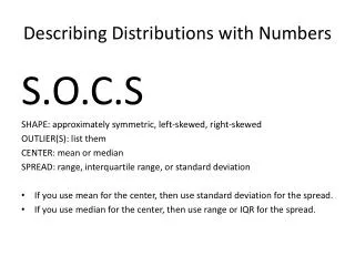
Comparing the Mean and the Median • The mean and median measure center in different ways, and both are useful. • Mean: “average” value Median: “typical” value • Relationship between Mean & Median: • The mean and median of a roughly symmetric distribution are close together. • If the distribution is exactly symmetric, the mean and median are exactly the same. • In a skewed distribution, the mean is usually farther out in the long tail than is the median.
Why is the mean more affected by the presence of outliers than the median?
Standard Deviation Standard deviation is a number used to tell how measurements for a group are spread out from the mean.
Standard Deviation • A relatively low standard deviation value indicates that the data points tend to be very close to the mean. • A relatively high standard deviation value indicates that the data points are spread out over a large range of values.
Standard Deviation Formula The standard deviationsxmeasures the average distance of the observations from their mean. It is calculated by finding an average of the squared distances and then taking the square root. This average squared distance is called the variance.
FYI: Why n-1?! Applet: http://www.uvm.edu/~dhowell/SeeingStatisticsApplets/N-1.html Proof
How to Calculate Standard Deviation by Hand • Calculate mean. • Calculate each deviation. Subtract your mean score from every actual (observed) score. • Square each deviation. • Find the “average” squared deviation by calculating the sum of the squared deviations divided by (n-1). 4. Divide that sum by the number of cases in your data 5. Finally, calculate the square root of the number calculate in step #4
Calculate the Standard Deviation Calculate the standard deviation.
Calculate the Standard Deviation • Calculate the mean. • Step 1: 5 • Calculate each deviation. • deviation = observation – mean deviation: 1 - 5 = -4 deviation: 8 - 5 = 3 = 5
Calculate the Standard Deviation 3) Square each deviation. Step 3: See Table 4) Find the “average” squared deviation by calculating the sum of the squared deviations divided by (n-1). Step 4: “Average” squared deviation = 52/(9-1) = 6.5 Variance = 6.5
Calculate the Standard Deviation 5) Calculate the square root of the variance…this is the standard deviation. Step 5: Square root of variance Standard Deviation = 2.55
Two Extreme Examples: • In dataset #1, we have five people that report eating 4 pieces of cake and five people that report eating 6 pieces of cake, for a mean of 5 pieces of cake ([4+4+4+4+4+6+6+6+6+6]/10=5). • Mean =5; Variance = 1 • In dataset #2, we have five people that report eating 0 piece of cake and five people that report eating 10 pieces of cake, for a mean of 5 pieces of cake ([0+0+0+0+0+10+10+10+10+10]/10=5). • Mean = 5; Variance = 5
Below are dotplots of three different distributions, A, B, and C. Which one has the largest standard deviation? Justify your answer.
TI-NSpire: Calculate standard deviation and mean. 1. Select “Lists & Spreadsheet” (blue/green button at bottom of home screen) 2. Type the values into list1. 3. With your cursor on the values, press menu 4. Select 4: Statistics, then 1: Stat Calculations, press enter. 5. Select 1: One-Variable Stats
TI-NSpire: Calculate standard deviation and mean. • Set screen to: and then press enter.
Mean Standard Deviation
Interquartile Range (IQR) • To calculate: • Arrange the observations in increasing order and locate the median M. • The first quartile Q1is the median of the observations located to the left of the median in the ordered list. • The third quartile Q3is the median of the observations located to the right of the median in the ordered list. • The interquartile range (IQR) is defined as: • IQR = Q3 – Q1
Find and Interpret the IQR… Travel times to work for 20 randomly selected New Yorkers
Find and Interpret the IQR… Travel times to work for 20 randomly selected New Yorkers M = 22.5 Q3= 42.5 Q1= 15 IQR = Q3 – Q1 = 42.5 – 15 = 27.5 minutes Interpretation: The range of the middle half of travel times for the New Yorkers in the sample is 27.5 minutes.
Identifying Outliers In addition to serving as a measure of spread, the interquartile range (IQR) is used as part of a rule of thumb for identifying outliers. 1.5 x IQR Rule for Outliers Call an observation an outlier if it falls more than 1.5 x IQR above the third quartile or below the first quartile.
In the New York travel time data, we found Q1=15 minutes, Q3=42.5 minutes, and IQR=27.5 minutes. Calculate the outlier cutoffs using the IQR rule.
In the New York travel time data, we found Q1=15 minutes, Q3=42.5 minutes, and IQR=27.5 minutes. Calculate the outlier cutoffs using the IQR rule. For these data, 1.5 x IQR = 1.5(27.5) = 41.25 Q1 - 1.5 x IQR = 15 – 41.25 = -26.25 Q3+ 1.5 x IQR = 42.5 + 41.25 = 83.75 Any travel time shorter than -26.25 minutes or longer than 83.75 minutes is considered an outlier.
The Five-Number Summary The five-number summary of a distribution consists of the smallest observation, the first quartile, the median, the third quartile, and the largest observation, written in order from smallest to largest. Minimum Q1 M Q3 Maximum
TI- Nspire: 5 Number Summary 1. Select “Lists & Spreadsheet” (bottom of home screen) 2. Type the values into list1. 3. With your cursor on the values, press menu 4. Select 4: Statistics, then 1: Stat Calculations, press enter. 5. Select 1: One-Variable Stats
TI- Nspire: 5 Number Summary • Set screen to: and then press enter. 7. Scroll down to see the 5 number summary.
Boxplots (Box-and-Whisker Plots) • Draw and label a number line that includes the range of the distribution. • Draw a central box from Q1to Q3. • Note the median M inside the box. • Extend lines (whiskers) from the box out to the minimum and maximum values that are not outliers.
Construct a Boxplot Using our NY travel times data. Construct a boxplot.
Construct a Boxplot Using our NY travel times data. Construct a boxplot. M = 22.5 Max=85 Recall, this is an outlier by the 1.5 x IQR rule Q1= 15 Min=5 Q3= 42.5