Chapter 5 Probability Distributions

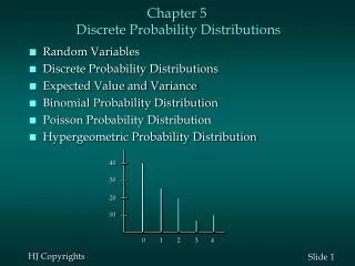
Chapter 5Probability Distributions 5-1 Review and Preview 5-2 Probability Distributions 5-3 Binomial Probability Distributions 5-4 Parameters for Binomial Distributions 5-5 Poisson Probability Distributions

Review and Preview This chapter combines the methods of descriptive statistics presented in Chapter 2 and 3 and those of probability presented in Chapter 4 to describe and analyze probability distributions. Probability distributions describe what will probably happen instead of what actually did happen, and they are often given in the format of a graph, table, or formula.

Preview In order to fully understand probability distributions, we must first understand the concept of a random variable, and be able to distinguish between discrete and continuous random variables. In this chapter we focus on discrete probability distributions. In particular, we discuss binomial and Poisson probability distributions.

Combining Descriptive Methods and Probabilities In this chapter we will construct probability distributions by presenting possible outcomes along with the relative frequencies we expect.

Key Concept This section introduces the important concept of a probability distribution, which gives the probability for each value of a variable that is determined by chance. Give consideration to distinguishing between outcomes that are likely to occur by chance and outcomes that are “unusual” in the sense they are not likely to occur by chance.

Random VariableProbability Distribution Random Variablea variable (typically represented by x) that has a single numerical value, determined by chance, for each outcome of a procedure Probability Distributiona description that gives the probability for each value of the random variable, often expressed in the format of a graph, table, or formula

Discrete and Continuous Random Variables Discrete Random Variableeither a finite number of values or countable number of values, where “countable” refers to the fact that there might be infinitely many values, but that they result from a counting process • Continuous Random Variablehas infinitely many values, and those values can be associated with measurements on a continuous scale without gaps or interruptions.

Probability Distribution: Requirements There is a numerical random variable x and its values are associated with corresponding probabilities. The sum of all probabilities must be 1. Each probability value must be between 0 and 1 inclusive.

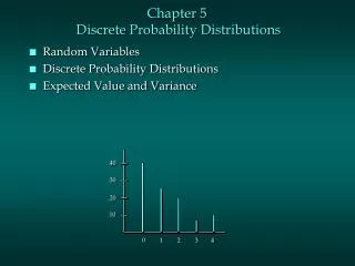
Graphs The probability histogram is very similar to a relative frequency histogram, but the vertical scale shows probabilities.

Mean Variance Variance (shortcut) Standard Deviation Mean, Variance and Standard Deviation of a Probability Distribution

Expected Value The expected value of a discrete random variable is denoted by E, and it represents the mean value of the outcomes. It is obtained by finding the value of

Example The following table describes the probability distribution for the number of girls in two births. Find the mean, variance, and standard deviation.

Identifying Unusual Results Range Rule of Thumb According to the range rule of thumb, most values should lie within 2 standard deviations of the mean. We can therefore identify “unusual” values by determining if they lie outside these limits: Maximum usual value = Minimum usual value =

Example – continued We found for families with two children, the mean number of girls is 1.0 and the standard deviation is 0.7 girls. Use those values to find the maximum and minimum usual values for the number of girls.

Identifying Unusual Results Probabilities Rare Event Rule for Inferential Statistics If, under a given assumption (such as the assumption that a coin is fair), the probability of a particular observed event (such as 992 heads in 1000 tosses of a coin) is extremely small, we conclude that the assumption is probably not correct.

Identifying Unusual Results Probabilities Using Probabilities to Determine When Results Are Unusual • Unusually high: x successes among n trials is an unusually high number of successes if . • Unusually low: x successes among n trials is an unusually low number of successes if .

Key Concept This section presents a basic definition of a binomial distribution along with notation and methods for finding probability values. Binomial probability distributions allow us to deal with circumstances in which the outcomes belong to two relevant categories such as acceptable/defective or survived/died.

Binomial Probability Distribution A binomial probability distribution results from a procedure that meets all the following requirements: 1. The procedure has a fixed number of trials. 2. The trials must be independent. (The outcome of any individual trial doesn’t affect the probabilities in the other trials.) 3. Each trial must have all outcomes classified into twocategories (commonly referred to as success and failure). 4. The probability of a success remains the same in all trials.

Notation for Binomial Probability Distributions (p = probability of success) (q = probability of failure) S and F (success and failure) denote the two possible categories of all outcomes; p and q will denote the probabilities of S and F, respectively, so

Notation (continued) n denotes the fixed number of trials. x denotes a specific number of successes in n trials, so x can be any whole number between 0 and n, inclusive. p denotes the probability of success in one of the n trials. q denotes the probability of failure in one of the n trials. P(x) denotes the probability of getting exactly x successes among the n trials.

Caution • Be sure that x and p both refer to the same category being called a success. • When sampling without replacement, consider events to be independent if .

Example • When an adult is randomly selected, there is a 0.85 probability that this person knows what Twitter is. • Suppose we want to find the probability that exactly three of five randomly selected adults know of Twitter. • Does this procedure result in a binomial distribution? • Yes. There are five trials which are independent. Each trial has two outcomes and there is a constant probability of 0.85 that an adult knows of Twitter.

Methods for Finding Probabilities We will now discuss three methods for finding the probabilities corresponding to the random variable x in a binomial distribution.

Method 1: Using the Binomial Probability Formula where n = number of trials x = number of successes among n trials p = probability of success in any one trial q = probability of failure in any one trial (q = 1 – p)

Method 2: Using Technology STATDISK, Minitab, Excel, SPSS, SAS and the TI-83/84 Plus calculator can be used to find binomial probabilities. STATDISK MINITAB

Method 2: Using Technology STATDISK, Minitab, Excel and the TI-83 Plus calculator can all be used to find binomial probabilities. EXCEL TI-83 PLUS Calculator

Method 3: Using Table A-1 in Appendix A Part of Table A-1 is shown below. With n = 12 and p = 0.80 in the binomial distribution, the probabilities of 4, 5, 6, and 7 successes are 0.001, 0.003, 0.016, and 0.053 respectively.

Strategy for Finding Binomial Probabilities • Use computer software or a TI-83/84 Plus calculator, if available. • If neither software nor the TI-83/84 Plus calculator is available, use Table A-1, if possible. • If neither software nor the TI-83/84 Plus calculator is available and the probabilities can’t be found using Table A-1, use the binomial probability formula.

Example Given there is a 0.85 probability that any given adult knows of Twitter, use the binomial probability formula to find the probability of getting exactly three adults who know of Twitter when five adults are randomly selected. We have: We want:

Example We have:

Rationale for the Binomial Probability Formula The number of outcomes with exactly x successes among n trials

Rationale for the Binomial Probability Formula The probability of x successes among n trials for any one particular order Number of outcomes with exactly x successes among n trials

Key Concept In this section we consider important characteristics of a binomial distribution including center, variation and distribution. That is, given a particular binomial probability distribution we can find its mean, variance and standard deviation. A strong emphasis is placed on interpreting and understanding those values.

Binomial Distribution: Formulas Mean Variance Std. Dev. Where n = number of fixed trials p = probability of success in one of the n trials q = probability of failure in one of the n trials

Interpretation of Results maximum usual value = minimum usual value = It is especially important to interpret results. The range rule of thumb suggests that values are unusual if they lie outside of these limits:

Example McDonald’s has a 95% recognition rate. A special focus group consists of 12 randomly selected adults. For such a group, find the mean and standard deviation.

Example - continued Use the range rule of thumb to find the minimum and maximum usual number of people who would recognize McDonald’s. If a particular group of 12 people had all 12 recognize the brand name of McDonald’s, that would not be unusual.

Key Concept The Poisson distribution is another discrete probability distribution which is important because it is often used for describing the behavior of rare events (with small probabilities).

Poisson Distribution The Poisson distribution is a discrete probability distribution that applies to occurrences of some event over a specified interval. The random variablex is the number of occurrences of the event in an interval. The interval can be time, distance, area, volume, or some similar unit. Formula

Requirements of thePoisson Distribution The random variable x is the number of occurrences of an event over some interval. The occurrences must be random. The occurrences must be independent of each other. The occurrences must be uniformly distributed over the interval being used. Parameters The mean is . • The standard deviation is

Differences from a Binomial Distribution The Poisson distribution differs from the binomial distribution in these fundamental ways: • The binomial distribution is affected by the sample size n and the probability p, whereas the Poisson distribution is affected only by the mean . • In a binomial distribution the possible values of the random variable x are 0, 1, . . ., n, but a Poisson distribution has possible x values of 0, 1, 2, . . . , with no upper limit.

Example • For a recent period of 100 years, there were 530 Atlantic hurricanes. Assume the Poisson distribution is a suitable model. • Find μ, the mean number of hurricanes per year. • If P(x) is the probability of x hurricanes in a randomly selected year, find P(2).

Example • Find μ, the mean number of hurricanes per year. • If P(x) is the probability of x hurricanes in a randomly selected year, find P(2).

Poisson as an Approximation to the Binomial Distribution Rule of Thumb to Use the Poisson to Approximate the Binomial The Poisson distribution is sometimes used to approximate the binomial distribution when n is large and p is small.

Chapter 5 Probability Distributions