Chapter 5 Probability Distributions

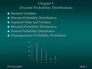
Chapter 5Probability Distributions 5-1 Overview 5-2 Random Variables 5-3 Binomial Probability Distributions 5-4 Mean, Variance and Standard Deviation for the Binomial Distribution 5-5 The Poisson Distribution

Section 5-1 Overview

This chapter will deal with the construction of discrete probability distributions by combining the methods of descriptive statistics presented in Chapter 2 and 3 and those of probability presented in Chapter 4. Probability Distributions will describe what will probably happen instead of what actually did happen. Overview

Combining Descriptive Methods and Probabilities In this chapter we will construct probability distributions by presenting possible outcomes along with the relative frequencies we expect.

Section 5-2 Random Variables

Key Concept This section introduces the important concept of a probability distribution, which gives the probability for each value of a variable that is determined by chance. Give consideration to distinguishing between outcomes that are likely to occur by chance and outcomes that are “unusual” in the sense they are not likely to occur by chance.

Random variable a variable (typically represented by x) that has a single numerical value, determined by chance, for each outcome of a procedure Probability distribution a description that gives the probability for each value of the random variable; often expressed in the format of a graph, table, or formula Definitions

Example 12 Jurors are to be randomly selected from a population in which 80% of the jurors are Mexican-American. If we assume that jurors are randomly selected without bias, here is an example of a probability distribution depicting these probabilities (let x = number of Mexican-American jurors among 12 jurors). Probabilities that are very small (such as 0.000000123) are represented by 0+.

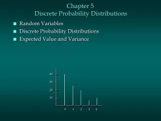
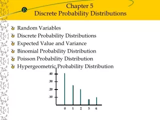
Graphs The probability histogram is very similar to a relative frequency histogram, but the vertical scale shows probabilities.

Discrete random variable either a finite number of values or countable number of values, where “countable” refers to the fact that there might be infinitely many values, but they result from a counting process. Example: Count of number of movie patrons Definitions • Continuous random variable infinitely many values, and those values can be associated with measurements on a continuous scale in such a way that there are no gaps or interruptions. Example: The measured voltage of a smoke detector battery.

The number of eggs a hen lays The count of the number of stats students present in class today The amount of milk a cow produces in one day The measure of voltage for a particular smoke detector battery Continuous or discrete?

 P(x) = 1 where x assumes all possible values. Requirements for Probability Distribution • 0 P(x) 1 • for every individual value of x.

Does this table describe a probability distribution? Does P(x) = x/3 (where x can be 0, 1, or 2) determine a probability distribution? Example

µ=[x•P(x)] Mean 2=[(x –µ)2 • P(x)] Variance 2=[x2 • P(x)] –µ2Variance (shortcut) = [x2 • P(x)] –µ2Standard Deviation Mean, Variance and Standard Deviation of a Probability Distribution

Round results by carrying one more decimal place than the number of decimal places used for the random variable x. If the values of xare integers, round µ, ,and2 to one decimal place. Roundoff Rule for µ,,and2

Identifying Unusual Results Range Rule of Thumb According to the range rule of thumb, most values should lie within 2 standard deviations of the mean. We can therefore identify “unusual” values by determining if they lie outside these limits: Maximum usual value = μ + 2σ Minimum usual value = μ – 2σ

The table below describes the prob. dist. for the number of Mexican-Americans among 12 randomly selected jurors in Hidalgo County, Texas. Assuming that we repeat the process of randomly selecting 12 jurors and counting the number of Mexican-Americans each time, find the mean number of Mexican-Americans (among 12), the variance, and the std. dev.

Identifying Unusual Results Probabilities Rare Event Rule If, under a given assumption (such as the assumption that a coin is fair), the probability of a particular observed event (such as 992 heads in 1000 tosses of a coin) is extremely small, we conclude that the assumption is probably not correct. • Unusually high: x successes among n trials is an unusually high number of successes if P(x or more) ≤ 0.05. • Unusually low: x successes among n trials is an unusually low number of successes if P(x or fewer) ≤ 0.05.

If 80% of those eligible for jury duty in Hidalgo County are Mexican-American, then a jury of 12 randomly selected people should have around 9 or 10 who are Mexican-American. Is 7 Mexican-American jurors among 12 an unusually low number? Does the selection of only 7 Mexican-Americans among 12 jurors suggest that there is discrimination in the selection process? Example

Definition The expected value of a discrete random variable is denoted by E, and it represents the average value of the outcomes. It is obtained by finding the value of  [x• P(x)]. E =  [x• P(x)] The mean of a discrete random variable is The same as its expected value!

If you bet $1 in Kentucky’s Pick 4 Lottery game, you either lose $1 or gain $4999 (the winning prize is $5000, but your $1 bet is not returned, so the net gain is $4999). The game is played by selected a four-digit number between 0000 and 9999. If you bet $1 on 1234, what is your expected value of gain or loss? Example

The random variable x is a count of the number of girls that occur when two babies are born. Construct a table representing the probability distribution, then find its mean and standard deviation. You do!

Recap In this section we have discussed: • Combining methods of descriptive statistics with probability. • Random variables and probability distributions. • Probability histograms. • Requirements for a probability distribution. • Mean, variance and standard deviation of a probability distribution. • Identifying unusual results. • Expected value.

Chapter 5 Probability Distributions