Download
1 / 24
240 likes | 398 Views
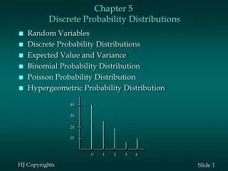
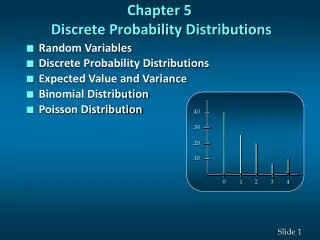
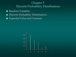
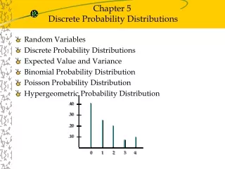
Chapter 5 Discrete Probability Distributions. Chapter Outline. Random Variables Discrete Probability Distributions Expected Value and Variance Binomial Probability Distribution. Random Variables. A random variable is a numerical description of the outcome of an experiment.

E N D
Chapter Outline • Random Variables • Discrete Probability Distributions • Expected Value and Variance • Binomial Probability Distribution
Random Variables • A random variable is a numerical description of the outcome of an experiment. • A discrete random variable assumes numerical values that have gaps or jumps between them. • A continuous random variable assumes numerical values that have NO gaps or jumps between them.
Random Variables Experiment Random Variable x Type Take a quiz with 10 Ture/False questions x = Number of correct answers Discrete x = time to finish a 5k run Run 5K Continuous Weigh a sample of 36 cans of coffee (labeled as 3lbs x = the average weight of a sample of 36 cans of coffee Continuous
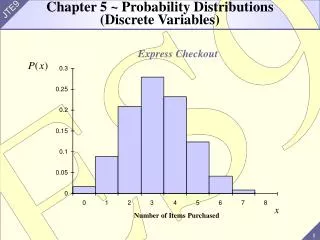
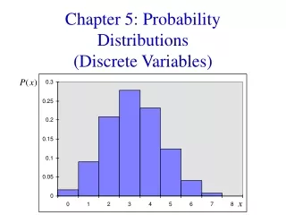
Discrete Probability Distributions • The probability distribution for a random variable describes how probabilities are distributed over the values of the random variable. • We can describe a discrete probability distribution with a table, graph, or formula.
Discrete Probability Distributions • The probability distribution is defined by a probability function, denoted by f(x), which provides the probability for each value of the random variable. • The required conditions for a discrete probability function are: f(x) > 0 f(x) = 1
Discrete Probability Distributions • Example: Probabilities of the # of correct answers to a quiz of 4 True/False questions. • We can use a table to represent the probability distribution. • The random variable x represents the number of correct answers. xf(x) 0 .10 1 .25 2 .35 3 .20 4 .10 1.00
Discrete Uniform Probability Distribution The discrete uniform probability distribution is the simplest example of a discrete probability distribution given by a formula. The discrete uniform probability function is f(x) = 1/n the values of the random variable are equally likely where: n = the number of values the random variable may assume
E(x) = = xf(x) Expected Value • The expected value, or mean, of a random variable is a measure of its central location. • The expected value is a weighted average of the values the random variable may assume. The weights are the probabilities. • The arithmetic mean introduced in Chapter 3 can be viewed as a special case of weighted average, where the weights for all the values are the same, i.e. 1/n.
Var(x) = 2 = (x - )2f(x) Variance and Standard Deviation • The variance summarizes the variability in the values of a random variable. • The variance is a weighted average of the squared deviations of a random variable from its mean. The weights are the probabilities. • The standard deviation, , is defined as the positive square root of the variance.
Expected Value • Example: Take a quiz (# of correct answers) xf(x)xf(x) 0 .10 .00 1 .25 .25 2 .35 .70 3 .20 .60 4 .10 .40 E(x) = 1.95 Expected number of correct answers
Variance • Example: Take a quiz (# of correct answers) x (x - )2 f(x) (x - )2f(x) x - 0 1 2 3 4 -1.95 -0.95 0.05 1.05 2.05 3.8025 0.9025 0.0025 1.1025 4.2025 .10 .25 .35 .20 .10 .3803 .2256 .0009 .2205 .4203 Variance of daily sales = s 2 = 1.2476 Standard deviation of daily sales = = 1.11 correct answers
Binomial Probability Distribution Properties of a Binominal Experiment: • The experiment consists of a sequence of n identical trials; • Only two outcomes, success and failure, are possible on each trial; • The probability of a success, denoted by p, does not change from trial to trial; • The trials are independent from one another.
Binomial Probability Distribution • Our interest is in the number of successes occurring in the n trials. • We let x denote the number of successes occurring in the n trials. • Either outcome can be named as ‘Success’. We need to make sure that in the calculation, the probability p is matched with the definition of the random variable x.
Binomial Probability Distribution • Binomial Probability Function where: x = the number of successes p = the probability of a success on one trial n = the number of trials f(x) = the probability of x successes in ntrials n! = n(n – 1)(n – 2) ….. (2)(1)
Binomial Probability Distribution • Binomial Probability Function Number of experimental outcomes providing exactly x successes in n trials Probability of a particular sequence of trial outcomes with x successes in n trials
Binomial Probability Distribution • Example: Purchasing a pair of shoes Based on recent sales data, a shoe store manager estimates that the probability a customer makes a purchase is 30%. For the next three customers, what is the probability that exactly 1 of them will make a purchase? Analysis: Is this example a binomial experiment? If so, which outcome is to be named ‘Success’? And what is the probability of Success?
Binomial Probability Distribution • Example: Purchasing a pair of shoes Does the example satisfy the properties of a binomial distribution? • N trials? – Yes, 3 trials ( 3 customers) • Two outcomes for each trial? – Yes, purchase or not • Probability of success stays the same – 30% chance for making a purchase can be assumed to be the same for all the customers. • Independent trials – Assume the three customers are independent in their decision on making a purchase.
Binomial Probability Distribution • Example: Purchasing a pair of shoes How many favorable outcomes are there where exactly ONE of the next three customers makes a purchase? With the success representing ‘making a purchase’ and the three customers assumed to be independent, we should have the following outcomes and their probabilities: Experimental Outcome (S, F, F) (F, S, F) (F, F, S) Probability of Experimental Outcome p(1 – p)(1 – p) = (.3)(.7)(.7) = .147 (1 – p)p(1 – p) = (.7)(.3)(.7) = .147 (1 – p)(1 – p)p = (.7)(.7)(.3) = .147 Total = .441
Binomial Probability Distribution • Example: Purchasing a pair of shoes Using the probability function Let: p = .30, n = 3, x = 1
Binomial Probability Distribution Example: Purchasing a pair of shoes Using a tree diagram x 2nd Customer 3rd Customer Prob. 1st Customer P (.3) .027 3 P (.3) .063 2 NP (.7) Purchase (.3) P (.3) .063 2 NP (.7) 1 .147 NP(.7) P (.3) 2 .063 P (.3) Not Purchase (.7) 1 .147 NP (.7) P (.3) 1 .147 NP (.7) 0 .343 NP (.7)
xf(x) 0 .343 1 .441 2 .189 3 .027 1.00 Binomial Probability Table • Statisticians have developed tables that give probabilities and cumulative probabilities for a binomial random variable. In the appendix of our textbook, you can locate the binomial probability tables. • For our example, the table is presented as below (where x represents the number of success):
Binomial Probability Distribution E(x) = = np • We can apply the formulas of expected value and variance for a binomial probability distribution. However, those formulas can be further simplified as follows: • Expected Value • Var(x) = 2 = np(1 -p) • Variance • Standard Deviation
Binomial Probability Distribution • Expected Value • Example: Purchasing a pair of shoes E(x) = np = 3(.3) = .9 customers out of 3 • Variance Var(x) = np(1 – p) = 3(.3)(.7) = .63 • Standard Deviation customers