Download
1 / 30
300 likes | 367 Views
Applications for Fine Resolution Marine Observations. Mark A. Bourassa 1,2,3 and Shawn R. Smith 1,3 1. Center for Ocean - Atmospheric Prediction Studies 2. Geophysical Fluid Dynamics Institute 3. The Florida State University bourassa@coaps.fsu.edu. General Applications.

E N D
Applications for Fine Resolution Marine Observations Mark A. Bourassa1,2,3 and Shawn R. Smith1,3 1. Center for Ocean-Atmospheric Prediction Studies 2. Geophysical Fluid Dynamics Institute 3. The Florida State University bourassa@coaps.fsu.edu
General Applications • Research vessel observations can be found in many regions of the globe, sampling a very wide range of conditions, which is ideal for all the many applications. • Modeling of surface turbulent fluxes (or radiation if it is measured). • Coupled with observations of surface turbulent fluxes (or co-located satellite data) the data are useful for evaluating and improving models of surface turbulent fluxes. • Comparison of time integrated fluxes to numerical weather prediction climate products. • Comparison to routine VOS data and assessment of quality of quality of VOS data. • Calibration or validation of satellite instruments. • Interpretation of errors in satellite data. • Useful for estimating naturally occurring noise in observations. NEW! NEW! Center for Ocean-Atmospheric Prediction Studies The Florida State University
Ocean’s TKE Based on Observed Surface Fluxes Eddy Correlation Inertial Dissipation Bulk Method Bulk Methods Calculations by Derrick Weitlich Clayson & Kanthamodel Center for Ocean-Atmospheric Prediction Studies The Florida State University
Flux Model Evaluation with ASTEX(Buoy Observations) Calculations by Yoshi Goto Center for Ocean-Atmospheric Prediction Studies The Florida State University
Observed Surface Stresses • Preliminary data form the SWS2 (Severe Wind Storms 2) experiment. • The drag coefficients for high wind speeds are large and plentiful. • The atypically large drag coefficients are associated with rising seas • Many models overestimate these fluxes. • Excellent empirical fit to means of these data and many other by P.K. Taylor & M. Yelland (2001). Center for Ocean-Atmospheric Prediction Studies The Florida State University
Evaluations Using SWS2 Ship and Buoy Observations All Data Stress < 0.5 N/m2 Calculations by Yoshi Goto Center for Ocean-Atmospheric Prediction Studies The Florida State University
Understanding Physics Via Differences in Remotely Sensed and In Situ Data In areas of strong currents, Uscat – Ubuoy will be dominated by the current. Areas with strong currents are often known, or can be identified in time series (Cornillon and Park 2001, GRL; Kelley et al. 2001, GRL). Remaining mean differences in Uscat – Ubuoy are expected to be dominated by wave-related variability in zo(u*) or ambiguity selection errors. • Problems related to ambiguity selection and dealing with vectors can be bypassed by comparing observed backscatter to the backscatter predicted by buoy observations (Bentamy et al. 2001, JTech). Center for Ocean-Atmospheric Prediction Studies The Florida State University
Comparison of Backscatter Residuals To Wave Parameters • Differences between observed and predicted (based on observed winds) backscatter are correlated with various wave parameter (Bentamy et al. 2001, JTech). • Significant wave height (the height of the 1/3 tallest waves) • Orbital velocity • Significant wave slope • Orbital velocity and significant slope are highly correlated. Correlation Coefficients Center for Ocean-Atmospheric Prediction Studies The Florida State University
Differences Between In Situ and Satellite Observations Could be Due to Physics • Surface stress modeling and QSCAT-derived stresses • Modeling surface stress for storm winds (Bourassa 2004 ASR) • Direct retrieval of surface turbulent stress from scatterometer backscatter Center for Ocean-Atmospheric Prediction Studies The Florida State University
Evaluations of Surface Fluxes in Climatologies • Quality processed R/V AWS data are ideal for evaluation of global reanalysis fluxes (e.g., Smith et al., 2001, J. Climate). • Sampling rates allow accurate estimation of 6 hourly integrated fluxes. Center for Ocean-Atmospheric Prediction Studies The Florida State University
Where are the Problems:Algorithm or Data • NCEP fluxes are compared to fluxes calculated from R/V data. • Fluxes calculated with Smith (1988) parameterization. • The triangles indicate a large bias that has a substantial dependence on wind speed. • Alternatively, fluxes can be calculated from the model winds, SST, air temperature, and atmospheric humidity (circles). • Much weaker dependence on wind speed. • Still a substantial bias. Center for Ocean-Atmospheric Prediction Studies The Florida State University
Evaluation of VOS Observation:VOSCLIM • Accuracies of VOS observations are not as well characterized as desired. • Wind biases have been studied in relatively great detail. • Lindau (1995) • CFD Modeling of flow distortion (Peter Taylor et al.) • Biases in SST have also beenexamined. • Biases in air temperature andatmospheric humidity are far lesswell know (Liz Kent). • Air temperature biases are expectedto be a function of radiative heatingand ventilation. Center for Ocean-Atmospheric Prediction Studies The Florida State University
Changes With Time As An Indication of Quality • Spikes, steps, suspect values identified (flagged) • Examines difference in near-neighbor values • Flags based on threshold derived from observations • Graphical Representation • Identifies flow conditions w/ severe problems • Flags plotted as function of ship-relative wind • % flagged in each wind bin on outer ring • Differences between ship and scatterometer could be used to examine flow distortion. Center for Ocean-Atmospheric Prediction Studies The Florida State University
R/V Data for Scatterometer ValidationCo-location Criteria • Automated Weather Systems • e.g., IMET • Observations interval is 5 to 60s • Record all parameters needed to calculate equivalent-neutral earth-relative winds • Co-location Criteria • Maximum temporal difference of 20 minutes (usually <30s). • Maximum spatial difference of 25 km (usually <12.5km). • Quality control includes checks for • Maneuvering (ship acceleration), • Apparent wind directions passing through superstructure. • Details in Bourassa et al. (2003 JGR) Center for Ocean-Atmospheric Prediction Studies The Florida State University
Collocations with R/V Atlantis Center for Ocean-Atmospheric Prediction Studies The Florida State University
Collocations with R/V Oceanus Center for Ocean-Atmospheric Prediction Studies The Florida State University
Collocations with R/V Polarstern Center for Ocean-Atmospheric Prediction Studies The Florida State University
Wind Speed Validation (QSCAT-1 GMF) • Preliminary results • 2 months of data • Observations from eight research vessels • <25 km apart,<20 minutes apart. • Uncertainty was calculated using PCA, assuming ships and satellite make equal contributions to uncertainty. Likely to be unflagged rain contamination Center for Ocean-Atmospheric Prediction Studies The Florida State University
R/V Atlantis Preliminary Comparison • Preliminary comparison to R/V Atlantis was much better than typical. • Uncertainties of 0.3 m/s and 4 (a factor of 4 or 5 better than average). • Possible explanations include a small sample, and • All but one co-location was <5 km. Center for Ocean-Atmospheric Prediction Studies The Florida State University
Variance in Speed • There have been several retrieval algorithms with different rain flags. • Ku2000 from Remote Sensing Systems. • QSCAT-1 from JPL. • Wind speed variance (i.e., uncertainty squared) decreases with decreasing co-location distance. Wind Direction Uncertainty2 (degrees2) Spatial Difference in Co-Location (km) Center for Ocean-Atmospheric Prediction Studies The Florida State University
Variance in Direction • Variance (uncertainty squared) in direction also decreases as co-location distance decreases. • Taylor’s hypothesis can be used to estimate the spatial scale to which extrapolation can be justified. • The optimum spatial scale is between 5 and 7 km. • This distance has been confirmed in the signal to noise ratio from backscatter (David Long, pers. Comm, 2003). Wind Direction Uncertainty2 (degrees2) Spatial Difference in Co-Location (km) Center for Ocean-Atmospheric Prediction Studies The Florida State University
Natural Variability In Scatterometer Observations • Examine how much noise in scatterometer winds is due to natural variability in surfaces winds. • Versus variability (noise) due to the retrieval function. • Will naturally variable winds be a serious problem for finer resolution scatterometer winds??? • Antenna technology has progressed to the point where a 1 or 2km product could be produced from a satellite in mid earth orbit. • Current scatterometer wind cells are 25x25km from low earth orbit. • There is a lot of atmospheric variability on scales <25km. • The different looks within a vector wind cell do not occur at the same time or location. The winds can and do change between looks. • These changes can be thought of as appearing as noise in the observed backscatter. When individual footprints are averaged over sufficient space/time (space in this case), the variability due to smaller scale processes can be greatly reduced. Center for Ocean-Atmospheric Prediction Studies The Florida State University
The Approach • Taylor’s hypothesis is used to convert a spatial scale (e.g., 25, 20, 15, 10, 5, and 2km) to a time scale. • Time scale = spatial scale / mean wind speed. • A maximum time scale of 40 minutes is used. • The non-uniform antenna pattern is considered. • The weighting in space (translated to time) is equal to a Gaussian distribution, centered on the center of the footprint, and dropping by one standard deviation at the edge of the footprint. • Mean speeds and directions are calculated, and differences are calculated for temporal differences of 1 through 20 minutes. Center for Ocean-Atmospheric Prediction Studies The Florida State University
Example of Variability in 60s Averagesfor Various Difference In Time • Variance in wind speed differences (m2s-2) as a function of the difference in time (minutes) for individual observations (one minute averages). 0 to 4 ms-14 to 8 ms-18 to 12 ms-112 to 16 ms-116 to 20 ms-1 Center for Ocean-Atmospheric Prediction Studies The Florida State University
Examples for 25km footprints • Standard deviation in wind speed differences (left; ms-1) and directional differences (right; degrees) as a function of the difference in time (minutes). • High wind speeds have more variability in speed, but less so in direction. • Directional variability for low wind speeds is very sensitive to the differences in time. Center for Ocean-Atmospheric Prediction Studies The Florida State University
Examples for 20km footprints • Standard deviation in wind speed (left; ms-1) and direction (right; degrees) as a function of the difference in time (minutes). Center for Ocean-Atmospheric Prediction Studies The Florida State University
Examples for 15km footprints • Standard deviation in wind speed (left; ms-1) and direction (right; degrees) as a function of the difference in time (minutes). Center for Ocean-Atmospheric Prediction Studies The Florida State University
Examples for 10km footprints • Standard deviation in wind speed (left; ms-1) and direction (right; degrees) as a function of the difference in time (minutes). • Odd features are creeping into the directional analysis for high wind speeds, presumably due to insufficient temporal resolution of the ship data. Center for Ocean-Atmospheric Prediction Studies The Florida State University
Examples for 5km footprints • Standard deviation in wind speed (ms-1) as a function of the difference in time (minutes). • Speeds, for large wind speeds, are highly sensitive to the differences in observation time. • For lower wind speeds, the spatial differences in sampling dominate the uncertainty in speed. Center for Ocean-Atmospheric Prediction Studies The Florida State University
Conclusions • There are many applications for high resolution in situ observations. • Improving flux modeling • Validation of climatologies • Quality assessment of VOS observations • Validation of satellite observations • Planning new earth observing satellites • The satellite related applications would benefit from observations with a sampling rate greater than once per minute. • Wave data and radiation data would be extremely useful for flux modeling. Center for Ocean-Atmospheric Prediction Studies The Florida State University