Download
1 / 30
300 likes | 395 Views
Statistical Analysis on the TI-83 Finding the mean, median, mode, standard deviation and range of a set of data. Press the STAT button, and select EDIT If data already exists in L1, you need to clear it. Up arrow until the L1 is highlighted Press the CLEAR button, then Enter

E N D
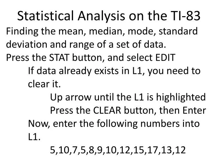
Statistical Analysis on the TI-83 Finding the mean, median, mode, standard deviation and range of a set of data. Press the STAT button, and select EDIT If data already exists in L1, you need to clear it. Up arrow until the L1 is highlighted Press the CLEAR button, then Enter Now, enter the following numbers into L1. 5,10,7,5,8,9,10,12,15,17,13,12
Statistical Analysis on the TI-83 Once the numbers have been entered, go to STAT again. If you are going to need to find the mode, you would want to sort the data. SORT A(, 2ND, 1 (to select L1), then Enter. It will say DONE. This will put the numbers into ascending order.
Statistical Analysis on the TI-83 Select STAT, then arrow to CALC enter 1, then press Enter 3 times This calculates 1-variable stats You will see the following information: x = 10.25 (this is the mean) ∑x = 123 (this is the sum of our list) ∑x2 = 1415 (we won’t use this) sx = 3.744693215 (stan. dev. of a sample) σx = 3.585270794 (stan. dev. of an entire population)
Statistical Analysis on the TI-83 n = 12 (number of items – sample space) Arrow down for more info!! Min X = 5 (smallest value) Q1 (median of top half of data) Med = 10 (median of all data) Q3 (median of bottom half of data) Max X = 17 (largest value) To find the range, simply subtract Min X from Max X (in our case, 17 - 5 = 12)
Statistical Analysis on the TI-83 The values that we will use for now are: x = 10.25 σx = 3.58 (rounded) MinX = 5 MaxX = 17
Stat – Edit – Enter numbers into L1 Stat – Calc – 1-Var stats Mean is 9.46 Standard Deviation (population) is 3.74
Apply to a Normal Distribution Applying this data to a normal distribution Also called a bell curve. 3.09 6.67 10.25 13.83 17.41 -3.58 -3.58 + 3.58 + 3.58 Standard Deviation Gap: Distance between each line from the mean
Apply to a Normal Distribution Percentages that hold for ALL normal distributions. 34.1% 34.1% 2.15% 13.6% 13.6% 2.15% 68.2% of data occurs between -1 and 1 s.d. 95.4% of data occurs between -2 and 2 s.d. 99.7% of data occurs between -3 and 3 s.d.
Apply to a Normal Distribution Z-Scores Used when we want to find the percentage of data above or below numbers that do not fall exactly on a standard deviation line. The number we are interested in minus the mean divided by the standard deviation.
Apply to a Normal Distribution Example: What percent of the data is below 7? 7 is not on a standard deviation line, so we need a z-score.
Apply to a Normal Distribution We have a z-score of -.91. We use this number on the z-score chart, which was given to you. Look for -.9 on the left, and .01 at the top. Where these intersect shows a value of .1814. The z-score table tells us what percentage of the data lies to the left of the number we are looking at.
Apply to a Normal Distribution This means that 18.14% of the data is to the left of (below) 7. Example: What percent of the data is above 14? 14 is not on a standard deviation line, so we need a z-score.
Apply to a Normal Distribution Using the z-score chart, look on the left side for 1.0, and then look at the top for .05. Where these intersect shows .8531. This means that 85.31% of the data is below14. Since we want to know what percentage is above 14, we need to subtract .8531 from 1. (1.00 - .8531 = .1469) 14.69% of the data should be above 14.
How do we know when to subtract the z-chart value, and when to just use it??? The z-score table gives us the percentage of data below the given number. If we want the percentage of data above that number, we have to subtract the table percentage from 1.00.
10.25 3.09 6.67 13.83 17.41 14 is higher than the mean, to its right. We are looking to the right of 14, so we are not crossing the mean. The answer must be less than 50%. Since the table gave us a value higher than 50%, we subtract it.
10.25 3.09 6.67 13.83 17.41 So, what did the table actually give us? It gave us the area LESS than 14. Looking at the curve, when looking at the area less than 14, we cross the mean. The value must be higher than 50%, which makes .8531 correct.
Normal Distribution Examples The heights of adult American males are normally distributed with a mean of 69.5 inches and a standard deviation of 2.5 inches. What percent of adult American males are between 67 and 74.5 inches tall? What are the z-scores? (67-69.5)/2.5 and (74.5-69.5)/500 -1 and 2 What percentage of data points lie between -1 and 2 standard deviations?
34.1 + 34.1 + 13.6 = 81.8% μ = 69.5 σ = 2.5 69.5 67.0 72.0 64.5 74.5
Normal Distribution In a group of 2000, about how many would you expect to be taller than 6 feet (72 inches)? What is the z-score? (72-69.5)/2.5 = ? z-score is 1. What percentage of data points will lie above 1 standard deviation from the mean? 15.75% of data will above that point
13.6 + 2.15 = 15.75% μ = 69.5 σ = 2.5 69.5 67.0 72.0 64.5 74.5
Normal Distribution In a group of 2000, about how many would you expect to be taller than 6 feet (72 inches)? Notice that question doesn’t ask for the percentage, it asks for the number of men out of a group of 2000. We would take the 2000 times the percentage to get our guess. 2000*.1575 = 315
Normal Distribution Josh’s and Richard’s Algebra II grades for the third cycle have the same mean (70). But Josh’s standard deviation is 15.6, and Richard’s is 20.1. What does the data tell us about their grades?
Richard σ = 20.1 Josh σ = 15.6 49.9 54.4 70 70 90.1 85.6 29.8 38.8 110.2 101.2 Josh was more consistent; Richard less so
Example 1: The weights of newborn humans are normally distributed about the mean, 3250 grams. The standard deviation is 500 grams. Find the probability that a baby chosen at random weighs between 2250 and 4250 grams. Step 1: Find the lower and upper z-scores. , The z-scores are -2 and 2.
Example 2: A company manufactures batteries having a lifespan that are normally distributed with a mean of 45 months and a standard deviation of 5 months. Find the probability that a battery chosen at random will have a lifespan of 50-55 months. Step 1: Find the lower and upper z-scores. , The z-scores are 1 and 2.
13.6% chance that the battery will have a lifespan between 50-55 months.
Need z-scores for 82 and 90. (82-72.3)/8.9 = 1.09 and (90-72.3)/8.9 = 1.99 The z-score chart tells us that .8621 of the data is below 82, and .9767 is below 90. We subtract (9767 - .8621) to get the % between the two scores, and then multiply by 184. 184*.1146 = 21.08, or 21 students.