Download
1 / 21
210 likes | 321 Views
Regional Processing. There goes the neighborhood. Rank Filtering. Rank filtering is a nonlinear process that is based on a statistical analysis of neighborhood samples.

E N D
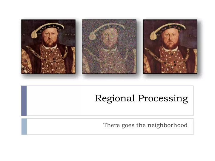
Regional Processing There goes the neighborhood
Rank Filtering • Rank filtering is a nonlinear process that is based on a statistical analysis of neighborhood samples. • Rank filtering is typically used, like image blurring, as a preprocessing step to reduce image noise in a multistage processing pipeline. • The central idea in rank filtering is to make a list of all samples within the neighborhood and sort them in ascending order. The term rank means just this, an ordering of sample values. The rank filter will then output the sample having the desired rank. • The most common rank filters are given as: • Median: The median sample • Minimum: The lowest-ranked sample • Maximum: The highest-ranked sample
Ranke Filtering: Median • Median filtering and averaging are similar but not identical • Median filtering is resistant to noise since a single noisy sample doesn’t affect the output. • Averaging is not as resistant to noise since a single noisy sample does affect the output. • Median filtering preserves edges that averaging blurs • Salt-and-Pepper noise occurs when samples of an image are incorrectly set to either the max (salt) or minimum (pepper) values. • Occurs in many CCD devices which have defective sites • Median filters excel at reducing salt and pepper noise
Comparison of Smoothing and Median Filtering with Salt and Pepper Noise
Rank Filtering Masks • Unlike most other regional processing techniques, rank filtering often uses non-rectangular regions where the most common of such regions are in the shape of either a plus (+) or a cross (x). • In this text, a rectangular mask is used to specify non-rectangular regions where certain elements in the region are marked as either included (white) or excluded (black) from the region.
Rank Filtering: Analysis • Computationally slow implementation. Assume an NxN rectangular region and a WxH source • Requires sorting NxN samples for each source sample • Assume that sorting N2 samples takes time proportional to N2*log(N2) • Filtering takes time proportional to WHN2*log(N2). Too slow! • Can improve performance by noting that: • Minimum/Maximum filtering doesn’t require sorting. • Can also improve performance by leveraging the fact that adjacent regions overlap. Use previous regions computational output to bootstrap the next region. • Can also use approximation based on successive Nx1 and 1xN rank filtering (similar to separability).
Median filtering approximation(3x3 row followed by column median filtering)
Median Filtering • A technique that leverages the computational overlap between successive regions.
Other Statistical Filters: Range • Range filtering is related to rank filtering but it is not itself a rank filter and hence cannot be accomplished directly by the RankOp class. • Range filtering produces the difference between the maximum and minimum values of all samples in the neighborhood such that it generates large signals where there are large differences (edges) in the source image and will generate smaller signals where there is little variation in the source image. • Implement using image subtraction with the min and max filtered images.
Other Statistical Filters: Most Common • Rather than keying on rank it is possible to select the most common element in the neighborhood. • This is a histogram-based approach that produces a distorted image where clusters of color are generated. The resulting image will generally have the appearance of a mosaic or an oil painting with the size and shape of the mask determining the precise effect. • If two or more elements are most common the one nearest the average of the region should be selected; otherwise choose the darker value. • It should be noted that performing this filter in one of the perceptual color spaces produces superior results since smaller color distortions are introduced.
Template Matching and Correlation • Consider the problem of locating an object in some source image. In the simplest case the object itself can be represented as an image which is known as a template. • A template matching algorithm can then be used to determine where, if at all, the template image occurs in the source. • One template matching technique is to pass the template image over the source image and compute the error between the template and the subimage of the source that is coincident with the template. A match occurs at any location where the error falls below a threshold value.
Template Matching and Correlation • Given source image f and an MxN template K where both M and N are odd, we can compute the RMS error g at location (x,y) as: • Minima in g denote likely matches to the template K.
Template Matching and Correlation • Correlation is similar to convolution • Better to normalize the correlated values where K-bar is the average of the template values and can be pre-computed. I-bar(x,y) is the average of all values in the region of I.