Download
1 / 34
340 likes | 457 Views
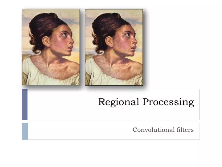
Regional Processing. Convolutional filters. Smoothing. Convolution can be used to achieve a variety of effects depending on the kernel. Smoothing, or blurring, can be achieved through convolution and is often used to reduce image noise or to prepare an image for further processing stages.

E N D
Regional Processing Convolutional filters
Smoothing • Convolution can be used to achieve a variety of effects depending on the kernel. • Smoothing, or blurring, can be achieved through convolution and is often used to reduce image noise or to prepare an image for further processing stages. • Smoothing is accomplished by any kernel where all of the coefficients are nonnegative. • Two classes of smoothing filters are commonly used. • Uniform filter: all non-zero coefficients are identical • Weighted (non-uniform) filter: Coefficients are larger near the center and smaller near the periphery.
Smoothing • The equations for • Pyramid: • Cone: • Gaussian: • Pyramid and Cone are non-smooth • Gaussian has desirable characteristics: • Smooth • Separable
Gaussian Smoothing • Gaussian is parameterized on the standard deviation • Large sigma’s reduce the center peak and spread the information across a larger area • Smaller sigma’s create a thinner and taller peak • Gaussian is separable – find A and B factors • Gaussian is radially symmetric which implies A = BT • Use the equation below where sigma controls the kernel shape and alpha controls the discrete kernel size where W = ceiling(alpha * sigma) and alpha is usually in [2,5].
Gaussian Smoothing • Consider generating a kernel using • Alpha = 2 • Sigma = 1 • Compute W = ceiling(2 * 1) = 2 • This is the half-width of the kernel. The kernel is then 5x5 • A and B are 5x1 and 1x5 respectively • Using the equation we obtain non-normalized A and B as • Normalized and rounded as {1, 4, 7, 4, 1}
Edges • An edges is a rapid transition between light and dark areas in an image. • Two common concerns: • Edge detection • Sharpening • The goal of edge detection is to identify locations in an image where the transition is strong. • Strong edges likely indicate component boundaries • Edges can be enhanced to sharpen an image • Blurring reduces the strength of edges while sharpening strengthens the edge strength. • Averaging is analogous to integration while sharpening is analogous to differentiation. • Derivative filters are usually used for edge detection • The derivative is a measure of color change over distance
Edges: Gradient • An edge is indicated by local extrema in the derivative • The derivative of a multi-variate function is known as the gradient and is a measure of the change that occurs in each dimension of the function. • Images are functions of two variables: (x, y) • The gradient measures both horizontal and vertical change • The gradient at a single location (x,y) is given as the 2x1 vector
Edges: Gradient • The gradient of the entire image is a table of such vectors and is known as a vector field. • The gradient is a vector and can be represented in either Cartesian coordinate space or polar coordinates. • Polar coordinates are a (radius, orientation) pair • Polar coordinates are often more useful since the coordinates directly correspond to edge strength (radius) and edge direction (orientation) • Conversion from Cartesian to Polar is straightforward:
Edges: Gradient • The gradient is a measure of the slope, or grade, at all points within the image. • Analogy: Consider a hiker who seeks to climb a hill by taking the most efficient path upwards. When standing at any point on the hill, the gradient • tells the hiker in which direction to take his next step (this is the orientation component) and • how much higher that step will take him (this is the r, or magnitude, component). • The gradient at a particular location is therefore a two- dimensional vector that points toward the direction of steepest ascent where the length (or magnitude) of the vector indicates the amount of change in the direction of steepest ascent. • The orientation of the gradient is therefore perpendicular to any edge that may be present.
Digital Approximation of the Gradient • Since digital images are not continuous but discrete, the gradient must be approximated rather than analytically derived. • Numerous methods for approximating the gradient of a discrete data set are in common use. Let’s start with a simple method • Consider a 3x3 region of an image having samples centered at Sc, where the subscript stands for the center, and the surrounding samples are positioned relative to the center as either up/down or left/right as indicated by the subscripts. Given this information, we would like to approximate the amount of change occurring in the horizontal and vertical directions at location (x, y) of image I.
Digital Approximation of the Gradient • What is the horizontal and vertical change at Sc? • Can approximate this change by:
Gradients via Convolution • The gradient can be approximated via convolution. Consider the kernels Gx and Gy which measure the horizontal and vertical changes:
Prewitt Operators • The previous approximations are noise-sensitive since a single noisy sample will greatly influence the gradient. • The Prewitt operators are kernels for use in convolution. • They average the difference across the central element and hence provide some immunity to noise.
Sobel Operators • Sobel operators both blur (average) and differentiates and image. • The operators are weighted with greater emphasis on the key element
Roberts Cross-Gradient operators • Measure change in the upper-left-to-bottom-right and bottom-left-to-upper-right diagonals rather than the horizontal and vertical axes. • Are 2x2 with the key element in the upper-left
Magnitude of Gradient • Edge detection algorithms typically key on the magnitude of the gradient (MoG) since larger magnitudes directly correspond to greater probability of an edge. • Computing the MoG is a fundamental building block in image processing. The MoG is defined in 6.18 • An edge map is the inverse of the MoG • Can detect edges by threshholding the MoG. Magnitudes above the threshold are assumed to be on an edge. • The MoG can be approximated as the sum of the horizontal and vertical magnitudes rather than the more computationally consuming sqrt of the sum-of-squares
MoG Implementation • Author a BufferedImageOp class to generate the magnitude of gradient from a source image. • Let’s use the first approach described in the text • Gx = [-1, 0, 1] and Gy = [-1, 0, 1]T
Edge Enhancement via Convolution • Edge enhancement is often known as sharpening. It boosts the high-frequency components of an image rather than suppressing the low-frequency components • Can be achieved via convolution but what kernel(s) should we use? • Consider that an image is the sum of the low and high frequency components • Boost the high-frequency component by a scaling factor alpha
Edge Enhancement via Convolution • Solve 6.20 for Ihigh and substitute into 6.21 • This equation can then be used to generate appropriate sharpening kernels • Assume that I = I convolved with Kidentityand Ilow = I convolved with Klow
Edge Enhancement via Convolution • The parameter alpha can be considered a gain setting that controls how much of the source image is passed through to the sharpened image. • When alpha= 0 no additional high frequency content is passed through to the output such that the result is the identity kernel. • Higher scaling factors correspond to stronger edges in the output.