Download
1 / 81
850 likes | 1.16k Views
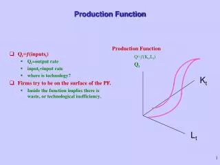
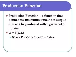
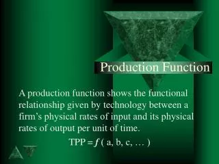
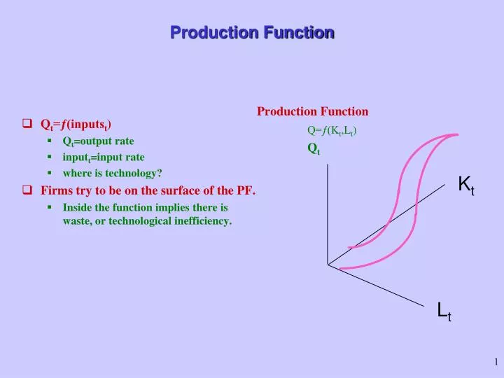
Q t =ƒ(inputs t ) Q t =output rate input t =input rate where is technology? Firms try to be on the surface of the PF. Inside the function implies there is waste, or technological inefficiency. Production Function Q=ƒ(K t ,L t ) Q t. Production Function. K t. L t.

E N D
Qt=ƒ(inputst) Qt=output rate inputt=input rate where is technology? Firms try to be on the surface of the PF. Inside the function implies there is waste, or technological inefficiency. Production Function Q=ƒ(Kt,Lt) Qt Production Function Kt Lt
Difference between LR and SR • LR is time period where all inputs can be varied. • Labor, land, capital, entrepreneurial effort, etc. • SR is time period when at least some inputs are fixed. • Usually think of capital (i.e., plant size) as the fixed input, and labor as the variable input.
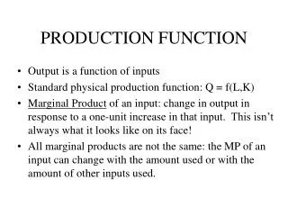
LR production function as many SR production functions. • Long Run: Q = f (K,L) • Suppose there are two different sized plants, K1 and K2. • One Short Run: • Q = f ( K1,L) i.e., K fixed at K1 • A second Short Run: • Q = f ( K2,L) i.e., K fixed at K2 • Show this graphically
Two Separate SR Production Functions Q Q = f( K2, L ) Q = f( K1, L ) K2 > K1 L
What Happens when Technology Changes? This shifts the entire production function, both in the SR and in the LR.
Technology Changes Q TP after computer TP before computer L
Express this in two dimensions, L and Q, since K is fixed. Define Marginal Product of Labor. Slope is MPL=dQ/dL Identify three ranges I: MPL >0 and rising II: MPL >0 and falling III: MPL<0 and falling I IIIII SR Production Function in More Detail Qt=ƒ(Kfixed,Lt) Q L
As you add more and more variable inputs to fixed inputs, eventually marginal productivity begins to fall. As you move into zone II, diminishing returns sets in! Why does this occur? Where Diminishing Returns Sets In Q I II L
Since plant size (i.e., capital) is fixed, labor has to start competing for the fixed capital. Even though Q still increases with L for a while, the change in Q is smaller. Why Diminishing Returns Sets In Q I II L
Define APL and MPL • Average Product = Q / L • output per unit of labor. • frequently reported in press. • Marginal Product =dQ/dL • output attributable to last unit of labor used. • what economists think of.
Take ray from origin to the SR production function. Derive slope of that ray Q=Q1 L=L1 Thus, Q/L =Q1 /L1 Average Productivity Graphically Q Q=f(KFIXED,L) Q1 • Q L L1 L
APL rises until L2 Beyond L2 , the APL begins to fall. That is, the average productivity rises, reaches a peak, and then declines Average Productivity Graphically Q Q=f(KFIXED,L) Q2 L Q/L L2 APL L2
Average & Marginal Productivity • There is a relationship between the productivity of the average worker, and the productivity of the marginal worker. • Think of a batting average. • Think of your marginal productivity in the most recent game. • Think of average productivity from beginning of year. • When MP > AP, then AP is RISING • When MP < AP, then AP is FALLING • When MP = AP, then AP is at its MAX
MPL rises until L1 Beyond L1 , the MPL begins to fall. Look at AP i. Until L2, MPL >APL and thus APL rises. ii. At L2, MPL=APL and thus APL peaks. iii. Beyond L2, MPL<APL and thus APL falls. Average Productivity Graphically Q L L1 L2 Q/L MPL APL L1 L2
Intuitive explanation • Anytime you add a marginal unit to an average unit, it either pulls the average up, keeps it the same, or pulls it down. • When MP > AP, then AP is rising since it pulls it the average up. • When MP < AP, then AP is falling since it pulls the average down. • When MP = AP, then AP stays the same. • Think of softball batting average example.
LR Production Function Qt Kt Isoquants (i.e.,constant quantity) Lt
Define Isoquant Different combinations of Kt and Lt which generate the same level of output, Qt.
Qt = Q(Kt, Lt) Output rate increases as you move to higher isoquants. Slope represents ability to tradeoff inputs while holding output constant. Marginal Rate of Technical Substitution. Closeness represents steepness of production hill. ISOQUANT MAP Isoquants & LR Production Functions K Q3 Q2 Q1 L
Slope is typicallynot constant. Tradeoff between K and L depends on level of each. Can derive slope by totally differentiating the LR production function. Marginal rate of technical substitution is –MPL/MPK Slope of Isoquant Kt Q Lt
No Substitutability Perfect Substitutability Extreme Cases K K Q2 Q2 Q1 Q1 L L Inputs used in fixed proportions! Tradeoff is constant
Low Substitutability High Substitutability Substitutability K K Q1 Q1 L L Slope of Isoquant changes a lot Slope of Isoquant changes very little
Isoquants and Returns to Scale Returns to scale are cost savings associated with a firm getting larger.
Production hill is rising quickly. Lines on the contour map get closer with equal increments in Q. Increasing Returns to Scale K Q=40 Q=30 Q=20 Q=10 L
Production hill is rising slowly. Lines on the contour map get further apart with equal increments in Q. Decreasing Returns to Scale K Q=40 Q=30 Q=20 Q=10 L
How Can You Tell if a PF has IRS, DRS, or CRS? • It is possible that it has all three, along various ranges of production. • However, you can also look at a special kind of function, called a homogeneous function. • Degree of homogeneity is an indicator returns to scale.
Homogeneous Functions of Degree • A function is homogeneous of degree k • if multiplying all inputs by , increases the dependent variable by • Q = f ( K, L) • So, • Q = f(K, L)is homogenous of degree k. • Cobb-Douglas Production Functions are homogeneous of degree +
Cobb-Douglas Production Functions • Q = A • K • L is a Cobb-Douglas Production Function • Degree of Homogeneity is derived by increasing all the inputs by • Q = A • (K) • (L) • Q = A • K • L • Q = A • K • L
Cobb-Douglas Production Functions • This is a Constant Elasticity Function • Elasticity of substitution s = 1 • Coefficients are elasticities is the capital elasticity of output, EK is the labor elasticity of output, E L • If Ek or L <1 then that input is subject to Diminishing Returns. • C-D PF can be IRS, DRS or CRS • if + 1, then CRS • if + < 1, then DRS • if + > 1, then IRS
Technical Change in LR • Technical change causes isoquants to shift inward • Less inputs for given output • May cause slope to change along ray from origin • Labor saving • Capital saving • May not change slope • Neutral implies parallel shift
Labor Saving Capital Saving K L Technical change K L
Lets now turn to the Cost Side What is Goal of Firm?
Put K on vertical axis, and L on horizontal axis. Assume input prices for labor (i.e., w) and capital (i.e., r) are fixed. Define: TC=w*L + r*K Solve for K: r*K= TC-w*L K=(TC/r) - (w/r)*L Isocost Line Define Isocost Line K Slope=-w/r TC/r L
TC constant along Isocost line. K TC1/r L TC1/w
in TC parallel shifts Isocost K TC2> TC1 TC2/r TC1/r L TC2/w TC1/w
Change in input price rotates Isocost K w2 < w1 TC/r L TC/w2 TC/w1
Suppose Optimal Output level is determined (Q1). Suppose w and r fixed. What is least costly way to produce Q1? Optimal Input Levels in LR K Q1 L
Suppose Optimal Output level is determined (Q1). Suppose w and r fixed. What is least costly way to produce Q1? Find closest isocost line to origin! Optimal point is point of allocative efficiency. Optimal Input Levels in LR K K1 Q1 L1 L
Cost Minimizing Condition • Slopes of Isoquant and Isocost are equal Slope of Isoquant=MRTS=- MPL/ MPK Slope of Isocost=input price ratio=-w/r At tangency, - MPL/ MPK =-w/r • Rearranging gives: MPL/w= MPK /r • In words: • Additional output from last $ spent on L = additional output from last $ spent on K.
Costs increase when output increases in LR! Look at increase from Q1 to Q2. Both Labor and Capital adjust. Connecting these points gives the expansion path. The LR Expansion Path K expansion path K2 K1 Q2 Q1 L L1 L2
We can show that LR adjustment along the expansion path is less costly than SR adjustment holding K fixed!
Start at an original LR equilibrium (i.e., at Q1). K K1 Q1 L L1
LR adjustment: K increases (K1 to K2) L increases (L1 to L2) TC increases from black to blue isocost. LR Adjustment K K2 K1 Q2 Q1 L L1 L2
SR adjustment. K constant at K1. L increases (L1 to L3) TC increases from black to white isocost. SR Adjustment K K1 Q2 Q1 L L1 L3
White Isocost (i.e., SR) is further from the origin than the Blue Isocost (LR). Thus, the more flexible LR is less costly than the less flexible SR. LR Adjustment less Costly K K2 K1 Q2 Q1 L L1 L2 L3
Start at equilibrium. Recall slope of isocost=K/L= -w/r Suppose w and optimal Q stays same (i.e., Q1) Rotate budget line out, and then shift back inward! Impact of Input Price Change K Q1 K1 L L1
Firms substitute away from capital (K1 to K2). Firms substitute toward labor (L1 to L2) Pure substitution effect: a to b Maps out demand for labor curve K a K1 b K2 Q1 L L1 L2 Decrease in wage leads to substitution
Wage falls w Derivation of Labor Demand from Substitution Effect K w1 a K1 w2 b K2 Q1 DL1 L1 L2 L L L1 L2
Scale effect is increase in output that results from lower costs Scale effect: b-c There is also a scale effect K Q1 Q2 a c K1 b L L1
Wage falls w Scale Effect Shifts Demand K w1 c a K1 w2 b K2 DL2 Q1 DL1 L1 L2 L3 L L L1 L2 L3
Recall the Isocost LineTC=w*L + r*K • Thus, TC=TVC+TFC • Lets relate the cost relationships to the production relationships. • Recall the Law of Diminishing Returns.