Download

1 / 30
300 likes | 436 Views
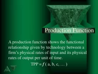
Chapter 9. Production Function, Factor Market and Aggregate Supply Function. Aggregate Supply Function. 1. Determinants of real income, employment and price. * AD and AS - What is a supply curve?. 2. AS Vs IS Curve.

E N D
Chapter 9 Production Function, Factor Market and Aggregate Supply Function
Aggregate Supply Function 1. Determinants of real income, employment and price *AD and AS - What is a supply curve? 2. AS Vs IS Curve a. Aggregate supply curve is flatter than the industry supply curve in the short-run • b. Aggregate supply curve is steeper than the industry supply curve in the long-run 3. Determinants of AS function * Potential output: Quantities and Qualities of inputs (production function) * Actual output: inputs and their prices, product price (shut down price)
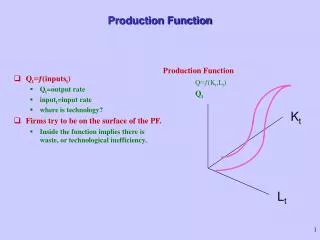
4. Production Function Y = f ( L , K ,T ) (9.1) f1 , f2 , f3 > 0 • Law of diminishing return (Non-linear prod. Function) • MPP of a factor varies directly with quantity of other • factors. Thus, labour productivity is higher in USA • than India
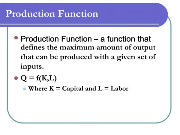
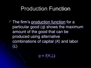
5.Labour/Capital Demand * Firms optimum behavior * Perfect competition in the product market Q = f (L, K) (9.2) C = L W + K R (9.3) Profit = TR – TC = f (L, K) P - L W – K R Optimisation would give MRP of labour = Marginal cost of labour MRP of capital = Marginal cost of capital
Under perfect condition, in both product and factor Market, the above conditions reduce to (9.4) MPP of labour = (9.5) MPP of capital = • Interdependence of production and factor demand functions Example: Q = A La K1-a (9.6) [(1-a) (Q/L)] / [a (Q/K)] = W/R L = [(1-a)/a]a [ R/W]a [ Q/A] (9.7) K = [a/(1-a)]1-a [W/R]1-a [Q/A] (9.8)
6. Labour Supply Function * Worker’s optimum behaviour - Income-Leisure trade-off Max. U = f(Y, L) f1, f2 > 0 Subject to Y = (T-L)(W/P) T = total time L = leisure *Backward bending labour supply curve: income and substitution effects.
* Shifts down if there is a. Increase in population b. Increase in work force participation rate c. Increase in working hours/day • d. liberalisation in immigration policy e. Increase in minimum wage f. Increase in retirement age g. Decrease in unemployment benefits • h. Increase in preference for work relative to leisure • => supply side economics ingredients
7. Capital Supply Function • Capital renters optimizing behaviour • Upward sloping • Shifts down if there is • a.Increase in propensity to save/invest b.Increase in the risk-preference of firms c. Increase in tax incentives for investment d. Liberalisation of foreign investments e. Improvement in property rights => supply side economics ingredients 8. Factor market equilibrium
Figure 9.4: Labour Market Equilibrium : Flex Wage (Classical) Real Wage D (MPP ) L L S L æ ö W ç ÷ è ø P 0 O L Labour 0 Full Employment
Figure 9.5 : Labour Market under Fixed Nominal Wage Rate ( Keynesian) Real Wage W0 / P2 W0 / P0 W0 / P1 DL Labour L0 L1 O L2
Price I II AS . . W 1 . W . 0 W . . 2 . . . Real Wage P Output 1 P 0 . . . P 2 (W/P) Y 0 F S L Y L F III IV Labour D L 9. AS Function: Lack of consensus • 9.1. AS curve under wage-price flexibility • Classical assumption Figure 9.6: ,
Implications • AS curve vertical at YF • Output is totally supply determined • Price and nominal wage directly and proportionally • related • Price is demand determined 9.2. AS curve under price rigidity (flex money/ real wage *Why fixed price? - Menu cost - Price contracts / brochures - Staggered price contracts - Competition on price front *Wage bargains in terms of money wage *Firms supply any output at the fixed price => firms ignore their labor demand curve
Figure 9.7 : AS Curve under Fixed Price Price I II B B’ W 1 AS W . 0 . . P0 A’ A . . . . . O Y0 Real Wage Output . . . L0 . . . (W/P) (W/P) Y 1 0 F S L L F Y IV III Labour
Implications • AS curve is inverted L - shaped • Mark up moves counter - cyclically • Nominal and real wage rates move pro-cyclical 9.3. AS curve under nominal wage rigidity (Flexible price) * Why nominal wage rigidity ? - Workers interested both in absolute and relative wage - Wage contracts - formal / informal, in money wage, not always indexed *Workers supply any labour at the fixed wage
Figure 9.8 : AS Curve under Nominal Wage Rigidity Price I II AS . . B . . P0 W A . . 0 . . C D . . . . . . . . P2 P1 P3 O Y3 Y2 Real Wage Output . . . . . L3 . . . . L2 . . Y L1 F W W W W 0 0 0 0 L F P P P P 1 3 2 0 Y III IV Labour D L
Implications Real wage movements counter cyclical SL= f(W/Pe) Workers suffer from money illusion Application U.K. data suggest that during 1929-36, U was high, money wage fell by 5% only initially, and even rose subsequently. Even W/P did not fall to clear U.
9.4. AS curve under Friedman-Lucas Information barrier * Asymmetric information: Worker’s fooling model AD↑ => Pˆ firms know workers do not => DLˆ => ASˆ * Information barrier ADˆ => Pˆ : Neither knows and each firm thinks the price of its product alone is up => DLˆ => ASˆ => AS is upward sloping
C Price . P0 B A . O Yn Output 9.5.Short and long run AS curves Figure 9.9 : a. P0BC is the short-run AS curve under the nominal price rigidity b. ABC is the short-run AS curve under the nominal wage rigidity/ fooling of workers/information barrier c. YFBC is the long-run AS curve under the full wage-price flexibility and perfect information.
10. Shifts in AS Function ( Supply shocks) * Could be caused by changes in a. labour force b. capital (structures, business equipment and inventories) c. materials and supplies d. energy resources and the level of e. technology (factor productivity) • f. weather conditions and, as we shall see later, g. expected inflation
11. AS Equation - Friedman -Lucas Version - Expected price augmented AS function (9.9) >0 * Slopes upward * Slope equals • * Position depends on Yn and Pe • Short-run function • In long-run • P = Pe and Y = Yn (9.10)
12. Phillips’ Curve Equation • W = f (ADL – ASL) • f1 > 0 • ADL = Labour employed + Vacancies • ASL = Labour employed + Unemployment. • ADL – ASL = - U *US estimates: 1950-66: w = - 1.43 + 8.27 (1/u) R2 = 0.38 For w = 0, u = 5.8 and w = 2, u = 2.4 At w = -1.43, u = infinity Incorporating un, : (9.11) • Un = NAIRU = LSUR • Two components of Un : Frictional U • Structural U
* Samuelson-Solow modification: (9.12) . - Permanent trade-off between P and u * Inflation-augmented (9.13) *Supply shock incorporated (9.14) * Short and long-run Phillips curve: temporary trade-off only * LP: correct expectations line * Overheated economy
Figure 9.10 : Phillips Curve LP Inflation Rate D E & P 2 e & & = SP ( P P ) 2 2 B C & P 1 e & & = SP ( P P ) 1 1 A & P 0 e & & = SP ( P P ) 0 0 O u u Unemployment Rate b n Position depends one to one on a. expected inflation rate, and b. adverse supply shock and negatively on • c. deviation of unemployment rate from its natural rate (= u-un = cyclical rate of unemployment)
13. Phillips’ curve vis a vis AS function Rewriting Phillips’ curve: Subtracting the lagged P gives
Treating these as log gives Okun’s law (Y-Yn) = f(u-un) f1<0 Or,
Phillips curve Substitution from the Okun’s law and inclusion of supply shock gives (9.15) • Same as AS function (9.9) • Trade off between growth and price stability
14. Adaptative Expectations’ Model • Sluggishness/ inertial in the economy • Backward looking theory = w1Pt + w2Pt-1+w3Pt-2 + .... = a Pt + a(1-a) Pt-1 + a(1-a)2 Pt-2 + .... (9.16) S = a + a(1-1) + a(1-a)2 + ..... = 1 = = a Pt-1 + a(1-a) Pt-2 + a(1-a)2 Pt-3 + ....
By subtracting the latter from the former, Or, (9.17) • Limitations • Systematic error prone • Ignore all other factors
15. Rational Expectations • Forward looking theory • Full information theory, expectation based on * current price * past prices * current and past values of all the variables which impinge on the price * expected/systematic policy actions and non-policy events which have bearings on the future price. * Smart use of the above information no formula but rational behaviour *May not get rightforecast but no systematic error • Limitations • No formula and thus subjective • Information cost and value
16. Conclusion * Allows price flexibility * Recognises resource constraint * Little consensus on AS curve