Download
1 / 15
150 likes | 188 Views
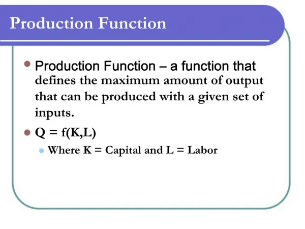
The Production Function II. 1. Costs - short run measures relationship - production & costs 2. Costs - long run scale expansion path long run costs 3. Returns to scale & economies of scale. 1. Costs - short run. Fixed & variable costs fixed = unavoidable variable = avoidable

E N D
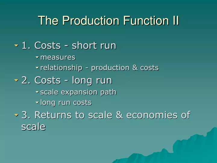
The Production Function II • 1. Costs - short run • measures • relationship - production & costs • 2. Costs - long run • scale expansion path • long run costs • 3. Returns to scale & economies of scale
1. Costs - short run • Fixed & variable costs • fixed = unavoidable • variable = avoidable • Costs rise as output increases • e.g. As L, TPP TC • given PK and PL • inverse relationship MP & MC, AC & AP • Measures of cost - Table 1
Measures of cost • Total costs: TC = TFC + TVC • Average costs: ATC = TC \ TPP • or TC \ Q • ATC = AFC + AVC • Marginal costs: MC =TC \ TPP • ‘…the extra cost of producing one more unit.’ • Shape - Figures 1 to 3
Total costs for firm X Output (Q) 0 1 2 3 4 5 6 7 TVC (£) 0 10 16 21 28 40 60 91 TC (£) 12 22 28 33 40 52 72 103 TFC (£) 12 12 12 12 12 12 12 12 TC TVC TFC fig
Average and marginal physical product b c Output APP MPP Quantity of the variable factor fig
Average and marginal costs MC Costs (£) x fig Output (Q)
2. Costs - long run • K & L are variable • Profit maximisation requires cost minimisation • Choice of technique: if • MPK \ PK > MPL \ PL • 20 \ 2 > 32 \ 8 • 10 > 4
Cost minimisation • i.e. last pound spent on K adds 10 units • Therefore • spend 1 extra pound on K, TPP rises by 10 • spend 2.50 less on L, TPP falls by 10 • output is unchanged, but costs fall 1.50 • Cost minimisation • MPK \ PK = MPL \ PL • tangency of isocost & isoquant
Scale expansion path & long run costs • Vary K & L TPP rises (no. of factories) • See Figure - scale expansion path • Long run average costs • Returns to scale • Scale economies
Deriving an LRAC curve from an isoquant map At an output of 100 LRAC = TC1 / 100 Units of capital (K) 100 O TC1 fig Units of labour (L)
Deriving an LRAC curve from an isoquant map Expansion path Units of capital (K) 700 600 500 400 300 200 100 O TC5 TC1 TC4 TC2 TC3 TC7 TC6 fig Units of labour (L)
A typical long-run average cost curve LRAC Costs O Output fig
Returns to scale • (i) Increasing returns • LRAC • a % increase in inputs leads to a larger % increase in output • economies of scale • (ii) Constant returns • LRAC constant • a given % increase in inputs leads to the same % increase in output
Returns to scale • (iii) Decreasing returns • LRAC • a % increase in inputs leads to a smaller % increase in output • diseconomies of scale • Economies of scale • plant level economies • multi-plant economies • Diseconomies of scale
Conclusion • Cost minimisation - long run • Profit = Revenue - Cost • Profit maximisation - level? • Market structure: • Perfect competition • Monopolistic competition • Oligopoly • Monopoly