Short-run Production Function

1. Short-run Production Function • Describes the technology that the firm uses to produce goods and services • E.g., • The more E and K the higher the firm’s output

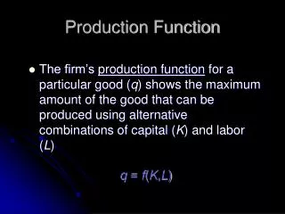
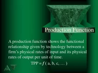
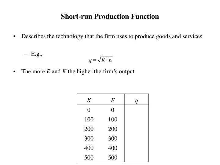
2. Short-run Production Function • Over the long-run K varies, but in the short-run K is fixed • E.g., K = 400 and • The more E the higher the firm’s short-run output

3. Law of diminishing marginal productivity • The marginal product of labor is (MPL) the change in output resulting from hiring an additional worker, holding constant the quantities of other inputs

4. Law of diminishing marginal productivity • The marginal product of labor is (MPL) the change in output resulting from hiring an additional worker, holding constant the quantities of other inputs

5. Law of diminishing marginal productivity • The marginal product of labor is (MPL) the change in output resulting from hiring an additional worker, holding constant the quantities of other inputs

6. Law of diminishing marginal productivity • The marginal product of labor is (MPL) the change in output resulting from hiring an additional worker, holding constant the quantities of other inputs

7. Law of diminishing marginal productivity • The marginal product of labor is (MPL) the change in output resulting from hiring an additional worker, holding constant the quantities of other inputs

8. The Total Product and Marginal Product curves Value If p = $1 per unit … w LD The total product curve gives the relationship between output and the number of workers hired by the firm (holding capital fixed). The marginal product curve gives the output produced by each additional worker, and the average product curve gives the output per worker. If we multiply each MPL value by p we get the VPL, the resulting graph is the firm’s labor demand.

9. Profit Maximization • Perfectly competitive firms cannot influence p, w, or r. Suppose p = 200, w = 70 and r = 30. In the short-run K is constant at say 100. • The short-run production function is • Fixed capital expenses: • Variable labor expenses • Total production expenses

10. Profit Maximization • Perfectly competitive firms cannot influence p, w, or r. Suppose p = 200, w = 70 and r = 30. In the short-run K is constant at say 100. • Revenue • Short-run profit

11. Profit Maximization TE Rev Slope Rev = Slope of TE VMP = w p∙MPL = w FE E The profit max condition: Slope profit = 0 E profit

12. Short-run Profit Maximization • Maximum profits occur when the profit curve reaches its peak (slope = 0) Profit maximizing employment Labor demand equation Slope of profit VMP = (0.5)(200)(10)E –0.5 = w

13. Labor Demand Curve • The demand curve for labor indicates how the firm reacts to wage changes, holding K = 100, r = 30, and p = 200 constant wage 70 40 20 204 625 2500 Employment

14. Labor Demand Curve • Recall VMP = (0.5)(200)(1000.5)E–0.5 = 1000E–0.5 • Since p = 200 andK = 100, the most general form of the labor demand curve is wage 70 40 20 204 319 1276 Employment

15. Profit Maximization Rules • The profit maximizing firm should produce up to the point where the cost of producing an additional unit of output (marginal cost) is equal to the revenue obtained from selling that output (marginal revenue) Choose q* so that MR = MC • Marginal Productivity Condition: this is the hiring rule, hire labor up to the point when the added value of marginal product equals the added cost of hiring the worker (i.e., the wage) Choose E* so that VMP = w

16. Long-run Production • In the long run, the firm maximizes profits by choosing how many workers to hire AND how much plant and equipment to invest in • Isoquant: describes the possible combinations of labor and capital that produce the same level of output, say at q0 = 500 units. • Isoquants… • Must be downward sloping • Cannot intercept • That are higher indicate more output • Are convex to the origin • slope is the negative ratio of MPK and MPL

17. Example: Isoquant curve with q0= 500 Isoquant curves 1250 capital 625 208 q0 = 500 200 400 1200 Employment

18. Example: Isoquant curve with q1= 600 Isoquant curves capital 900 300 q0 = 600 q0 = 500 200 400 1200 Employment

19. Isocost lines • The Isocost line indicates the possible combinations of labor and capital the firm can hire given a specified budget C0 = rK + wE C0 – wE = rK • Isocost indicates equally costly combinations of inputs • Higher isocost lines indicate higher costs

20. Isocost lines • Example: Suppose w = $70 per hour, r = $30 per hour, and C0 = $45,840. 1528 capital 1061 595 128 200 400600 Employment C0 = 45840

21. Isocost lines • Example: What happens if costs rise to C1 = $50,400 1680 1528 1213 capital 1061 747 595 128 128 C1 = 50400 200 400600 Employment C0 = 45840

22. Isocost lines • Example: When r = $30 • Example: What happens if r decreases to $27 C0 = 70(655) + 30(0) = $45,850 C0 = 70(655) + 27(0) = $45,850 1698 1528 capital 1179 1061 C0 = 45850 C0 = 45850 0 200 655 Employment

23. Isocost lines • Example: When w = $70 • Example: What happens if r decreases to $27 1528 C0 = 70(0) + 30(1528) = $45,840 C0 = 55(0) + 30(1528) = $45,840 1179 1061 capital C0 = 45840 C0 = 45840 327 200 655 Employment

24. Long-run cost minimization • Example: Suppose w = $70 per hour, r = $30 per hour, and q0 = 500 E* = 327 K* = 765 K C2 =70(204) +30(1200) = 50280 C* C1 = 70(327) + 30(765) = 45840 C0 = 70(204) + 30(834) = 39300 E

25. Long-run cost minimization • This least cost choice is where the isocost line is tangent to the isoquant • i.e., Marginal rate of substitution = w/r • Profit maximization implies cost minimization • The firm produces q0 = 500 units no matter what the K and E are. • The competitive firm is a price taker not a price maker (p = 91.68 was given) • Hence firm revenue = $45,840 no matter what the K and E are. • On the highest isocost line the firm would lose $4440 because C2 = 50280 • On the lowest isocost line the firm is unable to make 500 units • On the “just right” isocost line the breaks even because C* = $45,840.

26. Long Run Demand for Labor • If the wage rate drops, two effects take place • Firm takes advantage of the lower price of labor by expanding production (scale effect) • q can be increased at the same cost! • Firm takes advantage of the wage change by rearranging its mix of inputs (while holding output constant; substitution effect)

27. Example: Suppose w falls to 60 per hour Long Run Demand for Labor 1528 C* = 60(374) + 30(780) = $45,840 E* = 327 K* = 765 780 765 capital p = 91.68 Profit = $3667.20 C* = 45840 C* = 45840 327 Employment 374

28. Long Run Demand Curve for Labor Dollars When w = 70, E* = 327 When w = 60, E* = 374 70 60 DLR 374 327 Employment

29. Substitution and Scale Effects capital q1 q0 scale sub Employment

30. Elasticity of Substitution • The curvature of the isoquant measures elasticity of substitution • Intuitively, elasticity of substitution is the percentage change in capital to labor (a ratio) given a percentage change in the price ratio (wages to real interest) • This is the percentage change in the capital/labor ratio given a 1% change in the relative price of the inputs (w/r)

31. Imperfect substitutes in labor Black Labor An affirmative action program can encourage the discriminatory firm to minimize cost A discriminatory firm hires fewer blacks than what is optimal and hires more whites (it might have to import them!) Discriminatory firms production costs are higher than they would have been had they been color-blind q* White Labor

32. Imperfect substitutes in labor Black Labor An affirmative action program forces the color-blind firm to hire more blacks An affirmative action raises the color-blind firm’s production cost Which means the color-blind firm must hire fewer whites A color-blind firm hires relatively more whites because of the shape of the isoquants. q* White Labor

33. Other types of isoquants Capital and labor are perfect substitutes if the isoquant is linear. Hence, the firm can substitute two workers with one machine and not see its output change. The two inputs are perfect complements if the isoquant is right-angled. The firm then gets the same output when it hires 5 machines and 20 workers as when it hires 5 machines and 25 workers.