Download

1 / 25
250 likes | 346 Views
The impact of boundary layer dynamics on mixing of pollutants. Janet F.Barlow 1 , Tyrone Dunbar 1 , Eiko Nemitz 2 , Curtis Wood 1 , Martin Gallagher 3 , Fay Davies 4 and Roy Harrison 5 1 University of Reading 2 Centre for Ecology and Hydrology 3 University of Manchester

E N D
The impact of boundary layer dynamics on mixing of pollutants Janet F.Barlow1, Tyrone Dunbar1, Eiko Nemitz2, Curtis Wood1, Martin Gallagher3, Fay Davies4 and Roy Harrison5 1University of Reading 2Centre for Ecology and Hydrology 3University of Manchester 4University of Salford 5 University of Birmingham Funded by The BOC Foundation
Urban Boundary Layer dynamics: effect on aerosol distribution City scale: (from Oke, 1987)
Urban Boundary Layer dynamics: effect on aerosol distribution Neighbourhood scale: • heat and moisture sources / drag sinks are patchy • aerosol / precursor gas sources are patchy too! • vertical structure of turbulence and aerosols varies spatially and diurnally • Simultaneous measurements required • to attribute variability in pollutant concentrations • to both dynamical and chemical processes
Regents Park DAPPLE roof site BT Tower Lidar Site REPARTEE campaign 2007 Aim: Intensive observations of aerosols, trace gases and boundary layer dynamics to quantify variability in urban pollutants due to both chemical and meteorological processes. Special Issue in Atmospheric Chemistry and Physics! c. 1.6 km • Collaborators: Birmingham, York, Manchester, Salford (FGAM), Reading, CEH, Lancaster, Leicester, Cambridge, Environment Agency, Bristol
Doppler lidar measurements • Facility for Ground-based Atmospheric Measurement (FGAM) • 1.5 micron scanning Doppler lidar (Halo-photonics) • 24th Oct to 14th Nov 2007 • vertical stare • 30 m resolution gates • integration every 4 sec • backscatter • along beam Doppler velocity (vertical component)
R3 sonic anemometers (Gill) • 15th Oct to 15th Nov • 20Hz sampling frequency • height • z = 190 m (BT), 17 m (roof) • wind velocity, sonic temperature, fluxes Sonic anemometers
Influence of boundary layer on mixing • Big changes in: mixing height, • strength of turbulence, • vertical structure of turbulence • What is the impact on upward mixing of pollutants? • Estimate time taken to transport pollutant from street level up to BT Tower: • Simple approach! • z is height of BT Tower (190m) • w is standard deviation of vertical windspeed • ...compares well with REPARTEE tracer experiments • (see Martin et al. ACP, or Stock et al. poster)
Estimated time to diffuse from surface up to BT Tower Time (seconds)
Conclusions • Doppler lidar gives reliable measurements of turbulent structure of urban boundary layer • Lidar measurements indicate well-mixed profiles by day, separate layers of aerosol and turbulence at night of depth ~100-500m • Occasionally during night-time ground-level and BT Tower measurements can diverge, • i.e. the flow is decoupled from the surface • Mixing timescales depend on boundary layer turbulence • How far will pollutants be transported vertically (horizontally)? Latest work: Advanced Climate Technology Urban Laboratory (ACTUAL) Further Doppler lidar measurements in London • j.f.barlow@reading.ac.uk
Intercompare BT Tower and lidar • standard deviation of vertical velocity • big difference during calm, clear night • across all days, near 1:1 comparison • across all nights, lidar sometimes less than BT sonic, esp low values
Intercompare BT Tower and lidar • BT sonic resampled to 0.25 Hz to match lidar response • Lidar sampling rate “too slow” at night to capture small scale turbulence
Lidar observations – vertical velocity variance • hourly averages 6th Nov • normalised by convective velocity • where zi=BL depth • w’T’ = heat flux • θ = potential temp • Compare with Sorbjan (1991), CBL over homogeneous terrain • error bars = standard deviation • Peak below mid-boundary layer, indicating strong shear contribution to mixing
BT Tower observations • convective day, positive sensible heat flux, negative at night • clear skies throughout • northerly flow (i.e. from Park) • moderately strong winds
Intercompare sonic data at rooftop and BT Tower Rb ~ 0.1 • Despite statically stable conditions, Rb indicates turbulence still maintained at BT Tower so not completely decoupled
Windspeed during campaign Tracer
Figure 10: Example of stable conditions (2nd May). a) Mean and standard deviation of sonic temperature,
Fig 10 b) Ratio of virtual potential temperatures, and normalised turbulent kinetic energy at BT Tower and Lib sites. • www.dapple.org.uk