Download
1 / 20
280 likes | 537 Views
Observed Structure of the Atmospheric Boundary Layer. Many thanks to: Nolan Atkins, Chris Bretherton, Robin Hogan. Review of last lecture: Surface water balance. The changing rate of soil moisture S dS/dt = P - E - Rs - Rg + I. Precipitation (P). Evaportranspiration (E=Eb+Ei+Es+TR).

E N D
Observed Structure of the Atmospheric Boundary Layer Many thanks to: Nolan Atkins, Chris Bretherton, Robin Hogan
Review of last lecture: Surface water balance The changing rate of soil moisture S dS/dt = P - E - Rs - Rg + I Precipitation (P) Evaportranspiration (E=Eb+Ei+Es+TR) Irrigation (I) Runoff (Rs) dS/dt (PDSI, desertification) Infiltration (Rg)
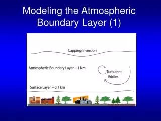
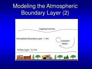
Vertical Structure of the Atmosphere • Definition of the boundary layer: "that part of the troposphere that is directly influenced by the presence of the earth's surface and responds to surface forcings with a time scale of about an hour or less.” • Scale: variable, typically between 100 m - 3 km deep
Difference between boundary layer and free atmosphere The boundary layer is: • More turbulent • With stronger friction • With more rapid dispersion of pollutants • With non-geostrophic winds while the free atmosphere is often with geostrophic winds
Vertical structure of the boundary layer From bottom up: • Interfacial layer (0-1 cm): molecular transport, no turbulence • Surface layer (0-100 m): strong gradient, very vigorous turbulence • Mixed layer (100 m - 1 km): well-mixed, vigorous turbulence • Entrainment layer: inversion, intermittent turbulence
Turbulence inside the boundary layer Definition of Turbulence: The apparent chaotic nature of many flows, which is manifested in the form of irregular, almost random fluctuations in velocity, temperature and scalar concentrations around their mean values in time and space.
Generation of turbulence in the boundary layer: Hydrodynamic instability “Hydrodynamically unstable” means that any small perturbation would grow rapidly to large perturbation • Shear instability: caused by change of mean wind in space (i.e. mechanical forcing) • Convective instability: caused by change of mean temperature in the vertical direction (i.e. thermal forcing)
Shear instability Shear: Change of wind in space
Example: Kelvin-Helmholtz instability Shear instability within a fluid or between two fluids with different density Lab experiment Real world (K-H clouds)
Convective instability • Static stability – refers to atmosphere’s susceptibility to being displaced • Stability related to buoyancy function of temperature • The rate of cooling of a parcel relative to its surrounds determines its ‘stability’ of a parcel • For dry air (with no clouds), an easy way to determine its stability is to look at the vertical profile of virtual potential temperature • v = (1 + 0.61 r ) • Where • = T (P0/P)0.286 is the potential temperature • r is the water vapor mixing ratio • Three cases: • (1) Stable (sub-adiabatic): v increases w/ height • (2) Neutral (adiabatic): v keeps constant w/ height • (3) Unstable (super-adiabatic): v decreases w/ height Stable or sub-adiabatic Neutral or adiabatic Unstable or super-adiabatic
Boundary layer stability conditions - Richardson number • The Richardson number is a convenient means of categorizing atmospheric stability in the boundary layer: Where g is acceleration due to gravity, is mean temperature, U is mean wind speed, z is height, and Ri is a dimensionless number. Ri >0 stable =0 neutral <0 unstable Lewis Fry Richardson (11 October 1881 - 30 September 1953) was an Englishmathematician, physicist, meteorologist, psychologist and pacifist who pioneered modern mathematical techniques of weather forecasting, and the application of similar techniques to studying the causes of wars and how to prevent them.
Forcings generating temperature gradience and wind shear, which affect the boundary layer depth • Heat flux at the surface and at the top of the boundary layer • Frictional drag at the surface and at the top of the boundary layer
Boundary layer depth:Effects of ocean and land • Over the oceans: varies more slowly in space and time because sea surface temperature varies slowly in space and time • Over the land: varies more rapidly in space and time because surface conditions vary more rapidly in space (topography, land cover) and time (diurnal variation, seasonal variation)
Boundary layer depth:Effect of highs and lows Near a region of high pressure: • Over both land and oceans, the boundary layer tends to be shallower near the center of high pressure regions. This is due to the associated subsidence and divergence. • Boundary layer depth increases on the periphery of the high where the subsidence is weaker. Near a region of low pressure: • The rising motion associated with the low transports boundary layer air up into the free troposphere. • Hence, it is often difficult to find the top of the boundary layer in this region. Cloud base is often used at the top of the boundary layer.
Boundary Layer depth:Effects of diurnal forcing over land • Daytime convective mixed layer + clouds (sometimes) • Nocturnal stable boundary layer + residual layer
Convective mixed layer (CML):Growth The turbulence (largely the convectively driven thermals) mixes (entrains) down potentially warmer, usually drier, less turbulent air down into the mixed layer
Convective mixed layer (CML):Vertical profiles of state variables Well-mixed (constant profile) Strongly stable lapse rate Nearly adiabatic Super-adiabatic
Nocturnal boundary layer over land: Vertical structure • The residual layer is the left-over of CML, and has all the properties of the recently decayed CML. It has neutral stability. • The stable boundary layer has stable stability, weaker turbulence, and low-level (nocturnal) jet. Weakly stable lapse rate Nearly adiabatic Strongly stable lapse rate
Boundary layer over land: Comparison between day and night Subtle difference between convective mixed layer and residual layer: Turbulence is more vigorous in the former Strongly stable lapse rate Nearly adiabatic Super-adiabatic Kaimal and Finnigan 1994 Weakly stable lapse rate Nearly adiabatic Strongly stable lapse rate
Summary • Vertical structure of the atmosphere and definition of the boundary layer • Vertical structure of the boundary layer • Definition of turbulence and forcings generating turbulence • Static stability and vertical profile of virtual potential temperature: 3 cases. Richardson number • Boundary layer over ocean • Boundary layer over land: diurnal variation