Download
1 / 36
390 likes | 588 Views
Frequency Domain Processing. Lecture: 3. 0. Overview of Linear Systems. In image processing, linear systems are at the heart of many filtering operations, and they provide the basis for analyzing complex problems in areas such as image restoration.

E N D
Frequency Domain Processing Lecture: 3
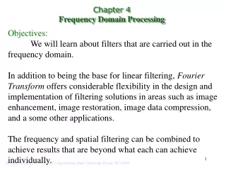
0. Overview of Linear Systems • In image processing, linear systems are at the heart of many filtering operations, and they provide the basis for analyzing complex problems in areas such as image restoration. • In this section we give a short review of linear systems
1The 2D Discrete Fourier Transform • Let f(x,y) for x=0,1,2, ..., M-1 and y=1,2, ..., N-1 denote an M×N image. The 2D DFT of f is given by • The frequency domain is simply the coordinate system spanned by F(u,v) with u and v as frequency variables.
1The 2D Discrete Fourier Transform • The inverse DFT is given by • Thus, givenF(u,v), we can obtain f(x,y) back by means of the inverse DFT.
1The 2D Discrete Fourier Transform • The value of the transform at the origin of the frequency domain that is F(0,0) is called the dc component of the Fourier transform. • Even if f(x,y) is real, its transform is complex. • The principal method of visually analyzing a transform is to compute its spectrum that is the magnitude of F(u,v).
1The 2D Discrete Fourier Transform • The Fourier spectrum is defined as • The phase angle is defined as
1The 2D Discrete Fourier Transform • The polar representation of F(u,v) is defined by • The power spectrum is defined as
1The 2D Discrete Fourier Transform It can be shown that The DFT is infinitely periodic in both u and v directions, with the periodicity determined by M and N.
1The 2D Discrete Fourier Transform Periodicity is also a property of the inverse DFT. An image obtained by taking the inverse DFT is also infinitely periodic in both u and v directions, with the periodicity determined by M and N.
2 Computing and Vizualizing the 2D DFT The FFT of an M × N image array is obtained by the syntax F=fft2(f) and with padding by the syntax F=fft2(f, P,Q) The Fourier spectrum is obtained as S=abs(F)
2 Computing and Vizualizing the 2D DFT The funcion F=fft2 (f) moves the origin of transform to the center of the frequency rectangle. Fc=fftshift (F) Log transformation: S2=log(1+abs(Fc)) Function ifftshift reverses the centering: F=ifftshift(Fc)
2 Computing and Vizualizing the 2D DFT To compute inverse FFT f=ifft2 (F) If the imput used to compute F is real then the inverse should also be real. However fft2 often has small imaginary components resulting from round-off errors. It is good practice to extract the real part of the result: f=real(ifft2(F))
3 Filtering in the frequency domain The convolution theorem: Linear spatial convolution is by convolving f(x,y) and h(x,y). The same result is obtained in the frequency domain by multiplying F(u,v) and H(u,v). The basic idea in frequency domain is to select a filter transfer function that modifies F(u,v) in a specified manner. A transfer function is multiplied by a centered F(u,v). A filter is called low pass filter if it attenuates the high frequency components to F(u,v) while leaving the low frequencies relatively unchanged.
3 Filtering in the frequency domain Example: Linear spatial filtering. f = 0 0 0 0 0 0 0 0 0 0 0 0 1 0 0 0 0 0 0 0 0 0 0 0 0 w = 1 2 3 4 5 6 7 8 9 g=imfilter(f, w, filtering_mode, boundary_options, size_options)
3 Filtering in the frequency domain g=imfilter(f, w, filtering_mode, boundary_options, size_options) >> g=imfilter(f,w,'corr',0,'full') g = 0 0 0 0 0 0 0 0 0 0 0 0 0 0 0 0 9 8 7 0 0 0 0 6 5 4 0 0 0 0 3 2 1 0 0 0 0 0 0 0 0 0 0 0 0 0 0 0 0
3 Filtering in the frequency domain With specified values of P and Q we use the following syntax to compute the FFT using zero padding. >> F=fft2(f, 7,7) F = Columns 1 through 2 1.00000000000000 -0.22252093395631 - 0.97492791218182i -0.22252093395631 - 0.97492791218182i -0.90096886790242 + 0.43388373911756i -0.90096886790242 + 0.43388373911756i 0.62348980185873 + 0.78183148246803i 0.62348980185873 + 0.78183148246803i 0.62348980185873 - 0.78183148246803i 0.62348980185873 - 0.78183148246803i -0.90096886790242 - 0.43388373911756i -0.90096886790242 - 0.43388373911756i -0.22252093395631 + 0.97492791218182i -0.22252093395631 + 0.97492791218182i 1.00000000000000 . . .
3.2 Basic steps in DFT filtering • Obtain the padding parameters P and Q. • Obtain the Fourier transform with padding: F=fft2(f, P,Q); • Generate a filter function, Hof sizeP×Q. If thefilter iscentered then use : H=fftshift(H)before using the filter. • Multiply the transform by the filter: G=H.*F; • Obtain the real part of G: g=real(ifft2(G)); • Crop the top,left rectangle to the original size: g=g(1:size(f,1), 1:size(f,2));
4. Lowpass frequency domain filters Ideal lowpassfilter (ILPF): where D(u,v) is the distance from point (u,v) to the center of the filter.
4. Lowpass frequency domain filters Butterworth lowpassfilter (ILPF): where D(u,v) is the distance from point (u,v) to the center of the filter.
4. Lowpass frequency domain filters Gaussian lowpassfilter (ILPF): where D(u,v) is the distance from point (u,v) to the center of the filter.