Download
1 / 67
680 likes | 710 Views
Chapter 4 Frequency Domain Processing. Objectives: We will learn about filters that are carried out in the frequency domain.

E N D
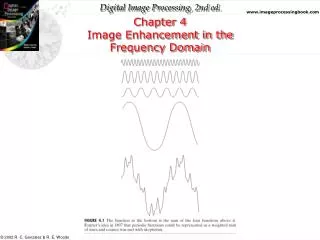
Chapter 4 Frequency Domain Processing Objectives: We will learn about filters that are carried out in the frequency domain. In addition to being the base for linear filtering, Fourier Transform offers considerable flexibility in the design and implementation of filtering solutions in areas such as image enhancement, image restoration, image data compression, and a some other applications. The frequency and spatial filtering can be combined to achieve results that are beyond what each can achieve individually.
Fourier Transform Fourier transform of a function f(x) (one-dimensional) is: where . We can obtain the f(x) using the inverse Fourier Transform. The two-dimensional version of this equations are: And the inverse Fourier Transform for this one can be shown as:
Discrete Fourier Transform To do any of these on a computer we need the discrete versions. For one dimensional case suppose we have M discrete points. In the two dimensional case, assume we have M and N discrete points in x and y directions respectively. One-dimensional: The inverse transform is:
Discrete Fourier Transform Two-dimensional: Where, f(x,y) denotes the input image with: x = 0, 1, 2, …, M-1 and y = 0, 1, 2, …, N-1 representing the number of rows and columns of the M-by-N image. The inverse transform is: Remember that we have: Since images are 2-D arrays, we work with these two.
What are they? The value of the transformation at the origin of the frequency domain [I.e., F(0,0)] is called the dc component of the Fourier Transform. F(0,0) is is equal to MN times the average value of f(x,y) Even if f(x,y) is real, it transformation in general is complex. To visually analyze a transform, we need to compute its spectrum. I.e., compute the magnitude of the complex variable F(u , v) and display it as an image. F(u,v) can also be represented as:
f(x,y) A y Y X x Discrete Fourier Transform Example Compute the Fourier transform of the function shown below:
Example – FFT Compute the FFT of f(x) = 2x. Let’s only computes for 4 frequencies.
F(2) = -1 F(3) = -1 - j
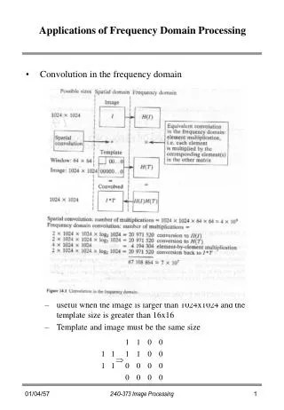
Example >> f = zeros(512,512); >> f(245:265,235:275)=1; >> imshow(f)
Example - cont >> F = fft2(f); >> F2 = log(abs(F)); >> imshow(F2)
Example – cont Centering the spectrum F = fft2(f); F2 = log(abs(F)); imshow(F2) for i = 1:512 for j = 1:512 f(i,j) = (-1)^(i+j)*f(i,j); end end F = fft2(f); F2 = log(abs(F)); figure,imshow(F2)
Filtering in the frequency domain In general, the foundation of linear filtering in both the spatial and frequency domains is the convolution theorem: Conversely, we will have: Here, the symbol “*” indicates convolution of the two functions, and the expression on sides of the double arrow denotes Fourier Transform pair. We are interested in the first one, where filtering in spatial domain consists of convoluting an image f(x,y) with a filter mask, h(x,y). Based on the convolution theorem we can obtain the same result by multiplying F(u,v) by H(u,v), the Fourier transform of the spatial filter. It is common to refer to H(u,v) as the filter transfer function.
Convolution and Correlation Example: Occurrences of a letter in a text
Read the Original Image, Store it in array text (Determine the size, Let’s say p, q) Read the image of the letter, Store it in an array l (Determine the size, Let’s say n, m) Rotate the image of the letter by 180 Compute the FFT of the letter, pad it to the p, q size Compute the FFT of the text
Multiply element-by-element the two Take the Real part of the result Multiply element-by-element the two Find the MAX Threshold based on the MAX Display
Based on convolution theorem: To obtain corresponding filtered image in the spatial domain we simply compute the inverse Fourier transform of the product of H(u,v)F(u,v). This is identical to what we would obtain by using convolution in the spatial domain, as long as the filter mask h(x,y) is the inverse Fourier transform of H(u,v). Convolving periodic functions can cause interference between adjacent period if the periods are close with respect to the duration of the nonzero parts of the functions.
This interference, wraparound error, can be avoided by padding the functions with zeros as explain below. Assume that functions f(x,y) and h(x,y) are of size AXB and CXD, respectively. Form two extended (padded)functions both of size PXQ by appending zeros to f and h. The wraparound error is avoided by choosing: In MATLAB, we will use F = fft2(f, PQ(1), PQ(2)) This appends enough zeros to f such that the resulting image is of size PQ(1)*PQ(2), then computes the FFT.
Basic Steps in DFT Filtering • Obtain the padding parameters using function paddedsize: • PQ = paddedsize(size(f)); • Obtain the Fourier transform with padding: • F = fft2(f, PQ(1), PQ(2)); • 3. Generate a filter function, H, of size PQ(1)XPQ(2) using one of the methods discussed in the remainder of this chapter. The filter must be in the format shown in Fig 4.4b. If it is not in that format, use shift to make it. • 4. Multiply the transform by the filter: G = H .* F
Basic Steps in DFT Filtering 5. Obtain the real part of the inverse FFT of G: g = real(ifft2(G)); 6. Crop the top, left rectangle to the original size: g = g(1:size(f, 1), 1:size(f, 2));
Example for DFT Filtering Try this for f = [0 0; 1 1]; PQ = paddedsize(size(f)); Fp = fft2(f, PQ(1), PQ(2)); HP = lpfilter(‘gaussian’, PQ(1), PQ(2), 2*sig); GP = HP .* Fp; gp = real(ifft2(GP)); gpc = gp(1:size(f,1), 1:size(f,2)); %cropping imshow(gp, [ ]) Similar result as: w = fspecial('gaussian', 3,3); gnew = imfilter(double(f), w)
Obtaining Frequency Domain Filters from Spatial Filters In general, filtering in the spatial domain is more efficient computationally than frequency domain filtering when the filters are small. One obvious approach for generating a frequency domain filter, H, that corresponds to a given spatial filter, h, is to let: H = fft2(h, PQ(1), PQ(2)), where the values of vector PQ depend on the size of the image we want to filter, as discussed in the last section. But we need to know:
Obtaining Frequency Domain Filters from Spatial Filters • How to convert spatial filters into equivalent frequency domain filters, • How to compare the results between spatial domain filtering using function imfilter, and frequency domain filtering.
F = fft2(f) S = fftshift(log(1+ abs(F))); S = gscale(S); imshow(S) 600x600 image
Generate the spatial filter using fspecial: h = fspecial(‘sobol’) h = 1 0 -1 2 0 -2 1 0 -1 To view a plot of the corresponding frequency domain filter:
PQ = paddedsize(size(f)); H = freqz2(h, PQ(1), PQ(2)); H1 = ifftshift(H); Origin at the top
Next, we generate the filtered images. In spatial domain we use: gs = imfilter(double(f), h); Which pads the border of the image with 0. The filtered image obtained by frequency domain processing: gf = dftfilt(f, H1); Download the dftfilt, paddedsize, and other related files from the notes web page.
gf = dftfilt(f, H1); Negative values are presented. Average is below the mid-gray value.
Using thresholding we can see the boundaries better abs(gs) > 0.2*abs(max(gs(:))))
Using thresholding we can see the boundaries better abs(gf) > 0.2*abs(max(gf(:))))
Generating Filters Directly in the Frequency Domain We discussed circularly symmetric filters that are specified as various functions of distance from the origin of the transform. One of the things we need to compute is the distance between any point and a specified point in the frequency rectangle. In MATLAB, for FFT computations the origin of the transform is at the top-left of the frequency rectangle. Thus, our distance is also measured from that point. In order for us to compute such a distance, we need the meshing system. This is what we call meshgrid array and is generated by dftuv function.
Example Here is an example of distance computation. In this example we will compute the distance squared from every point in a rectangle of size 8x5 to the origin of the frequency rectangle. >> [U , V] = dftuv(8, 5); This computes meshgrid frequency matrices U and V both of size 8-by-5. >> D = U.^2 + V.^2
U = 0 0 0 0 0 1 1 1 1 1 2 2 2 2 2 3 3 3 3 3 4 4 4 4 4 -3 -3 -3 -3 -3 -2 -2 -2 -2 -2 -1 -1 -1 -1 -1 V = 0 1 2 -2 -1 0 1 2 -2 -1 0 1 2 -2 -1 0 1 2 -2 -1 0 1 2 -2 -1 0 1 2 -2 -1 0 1 2 -2 -1 0 1 2 -2 -1
D = 0 1 4 4 1 1 2 5 5 2 4 5 8 8 5 9 10 13 13 10 16 17 20 20 17 9 10 13 13 10 4 5 8 8 5 1 2 5 5 2
U = 0 0 0 0 0 1 1 1 1 1 2 2 2 2 2 3 3 3 3 3 4 4 4 4 4 -3 -3 -3 -3 -3 -2 -2 -2 -2 -2 -1 -1 -1 -1 -1 V = 0 1 2 -2 -1 0 1 2 -2 -1 0 1 2 -2 -1 0 1 2 -2 -1 0 1 2 -2 -1 0 1 2 -2 -1 0 1 2 -2 -1 0 1 2 -2 -1 D = 0 1 4 4 1 1 2 5 5 2 4 5 8 8 5 9 10 13 13 10 16 17 20 20 17 9 10 13 13 10 4 5 8 8 5 1 2 5 5 2
function [U, V] = dftuv[M, N] u = 0: (M-1); v = 0: (N-1); idx = find(u > M/2); u(idx) = u(idx) – M; idy = find(v > N/2); v(idy) = v(idy) – N; [U, V] = meshgrid(u, v); The meshgrid function will produce two arrays. Rows on U are copies of rows in u and columns on V are copies of columns on v.
The distance with respect to the center of the frequency rectangle can be computed as: >> fftshift(D) ans = 20 17 16 17 20 13 10 9 10 13 8 5 4 5 8 5 2 1 2 5 4 1 0 1 4 5 2 1 2 5 8 5 4 5 8 13 10 9 10 13