Institute of Biophysics and Biomedical Engineering - Bulgarian Academy of Sciences

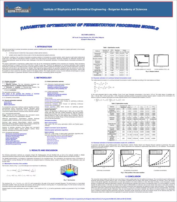
1. Institute of Biophysics and Biomedical Engineering - Bulgarian Academy of Sciences OLYMPIA ROEVA 105 Acad. George Bonchev Str. 1113 Sofia, Bulgaria olympia@clbme.bas.bg PARAMETER OPTIMIZATION OF FERMENTATION PROCESSES MODELS • 1. INTRODUCTION • Within the broad field of nonlinear fermentation processes systems modelling and management studies, the objective of global optimization is the analysis and application of [35]: • nonlinear decision models that (may) possess multiple optimal solutions; • suitable solution algorithms that are able to find the absolutely best (global) solution(s). • The dynamic modelling of the nonlinear fermentation processes systems is formulated as a reverse problem, which requires a well-suited mathematical model and a very efficient computational method to achieve the model structure and parameters. Numerical integration for differential equations and finding global parameter values are still two major challenges in this field of the parameter estimation of nonlinear dynamic fermentation processes (FP) systems. • The usage of optimization in engineering is getting larger every day as the computational capabilities of the computers are increasing. Today calculations could be performed in a fraction of the time it took just a couple of years ago. Therefore, the applications for numerical optimization have increased dramatically. A great part of the design process is and will always be intuitive; however analytical techniques as well as numerical optimization could be of great value and can permit vast improvement in designs. Real engineering design problems are generally characterized by the presence of many often conflicting and incommensurable objectives. This raises the issue about how different objectives should be combined to yield a final solution. There is also the question on how to search for an optimal solution to the design problem. This chapter presents a survey of some methods and techniques to conduct numerical optimization in a parameter estimation context and different ways of developing hybrids among them. Table 1. Optimization results a) time variation of x1 and x2 b) time variation of f(x1, x2) Fig. 2. Simplex method 2. METHODOLOGY 3.2. Parameter estimation of a nonlinear fed-batch fermentation model The mathematical formulation of a nonlinear fed-batch fermentation model is described according to the mass balance as follows: 2.1. Problem formulation 2.1.1. Basic ingredients 1. Objective function. The two interesting exceptions are: No objective function and Multiple objective functions. 2. Unknowns or variables. In fitting-the-data problem, the unknowns are the parameters that define the FP model. 3. A set of constraints. The optimization problem is then: Find values of the variables that minimize or maximize the objective function while satisfying the constraints. 2.1.2. Complexity of the problem 2.2. General optimization methods Local search Global search Global optimization For example the optimization methods could be classified as follows: Unconstrained versus Constrainedmethods; Derivative versus Non-derivativemethods; Deterministic versus Stochasticmethods; Local versus Globalmethods; Continuous versus Discretemethods. 2.2.1. Unconstrained optimization Newton method and some modifications like Line-search variant, Trust-region variant and Truncated Newton methods. Difference approximations, Quasi-Newton methods, Nonlinear conjugate gradient methods and the nonlinear Simplex method. Nonlinear least squares (Gauss-Newton method, Levenberg-Marquardtmethod and Hybrid methods (hybrid strategy combines the Gauss-Newton and BFGS Quasi-Newton algorithms)). Systems of nonlinear equations (Trust Region and Line-search methods, Truncated Newton method, Broyden method, Tensor methods, Homotopy and Continuation methods). 2.2.2. Constrained optimization Nonlinearly constrained optimization Bound-constrained optimization Quadratic programming Linear programming Simplex algorithm Interior-point algorithms Primal-dual interior-point algorithms Semidefinite programming 2.3. Global optimization methods 2.3.1. Elements of global optimization methods Strategies in choosing points Stopping conditions and solvability Convergence with probability one 2.3.2. Global optimization strategies Branch and bound Multistart and clustering methods Evolutionary algorithms These include: Genetic programming, which evolve programs; Evolutionary programming, which focuses on optimizing continuous functions without recombination; Evolutionary strategies, which focuses on optimizing continuous functions with recombination; Genetic algorithms(GAs), which focuses on optimizing general combinatorial problems. Genetic algorithms There is an abundance of different type of GAs such as simple GAs, steady stateGAs, GAs with multiple populations, GAs with crowding and sharing techniques, and many, many more.The different GAs have different features in order to solve different type of problems. GAs are very robust and can handle all type of fitness landscapes and mixture of real and discrete parameters. Simulated annealing Other meta-heuristics Tabu search (TS), Ant colony optimization (ACO), and Particle swarm methods. Adaptive stochastic search algorithms Statistical global optimization algorithms Hybrid methods There are a wide range of hybrid global optimization algorithms that have been developed. Some of hybrid algorithms are: Mixed Integer Nonlinear Programming (MINLP). Tree Annealing. Simulated annealing Pipelining hybrids. Asynchronous hybrids. Hierarchical hybrids. Additional operators. In this case generated data for state variables X and S are used. Substrate concentration in the feed is 100 g/l. The initial values of variables are: X(0)=1.25 g/l, S(0) = 0.81 g/l and V(0) = 1.35 l.Parameter estimation problem of presented nonlinear dynamic system is stated as the minimization of a distance measure J between generated and model predicted values of the considered state variables (X and S): Table 2. Optimization results (7) (8) ; 3.3. Parameter estimation of fed-batch fermentation model of E. coli MC4110 A parameter identification using Multipopulation GA, Quasi-Newton method, Simplex Search and Steepest Descentmethods is performed.The model predictions of the state variables, based on four sets of search parameters are compared to experimental data points of E. coli cultivation. The simulation results are presented in Fig. 3. 3. RESULTS AND DISCUSSION The following optimization methods are compared: Simple GA; Multipopulation GAand Modified GA; as well as the methods available in Matlab: Sequential quadratic programming method; Nelder-Mead Simplex method; BFGS Quasi-Newton method; Steepest descent and Minimax method. The Matlab implementation is considered of optimization procedures for all considered tests. The computations are performed using a PC/Pentium IV (3 GHz) platform running Windows XP. All methods are compared based on following criteria: number of iterations, CPU time, parameters value and function value. 3.1. Maximization a function of two variables Test function, shown on Fig. 1, is a 2-D landscape to be maximized. It is defined by: a) biomass concentrationb) substrate concentrationc) acetate concentration Fig. 3. Time profiles of the state variables 4. CONCLUSION The concurrent nature implies that GAs are much more likely to locate a global peak than the traditional techniques. The conventional search methods work extremely well provided it knows where to start. In the problem considered here the proper initial values of parameters are unknown. Due to the parallel nature of the genetic algorithm, the performance is much less sensitive to the initial conditions. In fact, GAs make hundreds, or even thousands, of initial guesses. Compared with traditional optimization methods, GA simultaneously evaluates many points in the parameter space. It is more probable to converge towards the global solution. A GA does not assume that the space is differentiable or continuous and can also iterate many times on each data received. A GA requires only information concerning the quality of the solution produced by each parameter set (objective function value information). This characteristic differs from optimization methods that require derivative information or, worse yet, complete knowledge of the problem structure and parameters. Since GAs do not demand such problem-specific information, they are more flexible than most search methods. Also GAs do not require linearity in the parameters which is needed in iterative searching optimization techniques. Simulation results reveal that accurate and consistent results can be obtained using GAs. The GAs property makes them suitable and more applicable for parameter estimation of fermentation processes models. Fig. 1. Test function The maximum f(х1, х2) = 1 is at (х1, х2) = (0.6, 0.1) and corresponds to the peak of the second, narrowed Gaussian. The test function is a hard global optimization problem. There are only two local maxima, with the global maximum covering about 1% of parameter space. For this function moving to the secondary maximum pulls solutions away from the global maximum. Detailed results of function optimization are given in Table 1. Time variations of f(x1, x2), as well as parameters variation are presented inFig. 2for Simplex method. ACKNOWLEDGEMENTS: The present work is supported by the Bulgarian National Science Fund grants № DMU 02/4, 2009 and DID 02-29/2009.