Download

1 / 30
300 likes | 400 Views
Unit 6: Standardization and Methods to Control Confounding. Unit 6 Learning Objectives: 1. Understand the “design” and “analysis” methods used to control confounding. --- Randomization --- Restriction --- Matching --- Stratification --- Multivariate analysis.

E N D
Unit 6: Standardization and Methods to Control Confounding
Unit 6 Learning Objectives: 1. Understand the “design” and “analysis” methods used to control confounding. --- Randomization --- Restriction --- Matching --- Stratification --- Multivariate analysis. 2. Understand pros and cons of the methods used to control confounding.
Lesson 6 Learning Objectives (cont.): 3. Understand the rationale for rate adjustment (standardization). 4. Apply and interpret the technique of direct standardization. 5. Apply and interpret the technique of indirect standardization. 6. Recognize differences between direct and indirect standardization.
Assigned Readings: Textbook (Gordis): Chapter 4, pages 60-68 (Age adjustment) Chapter 15, pages 230-232 (More on confounding) Hennekens and Buring: Evaluating the role of confounding. In Epidemiology in Medicine, pages 304-323.
CONFOUNDING - REVIEW DEFINITION: A third variable (not the exposure or outcome variable of interest) that distorts the observed relationship between the exposure and outcome. • Confounding is a confusion of effects that is a nuisance and should be controlled for if possible. • Age is a very common source of confounding.
CONFOUNDING - REVIEW E D Confounding IS present CF Confounding NOT present E ?CF D
CONFOUNDING Reason for controlling confounding: • To obtain a more precise (accurate) estimate of the true association between the exposure and disease under study. • As a general rule, age and gender should always be considered as potential confounders of an association.
CONFOUNDING POSITIVE CONFOUNDING: • The confounding factor produces an estimate that is more extreme (positive or negative) than the true association. NEGATIVE CONFOUNDING: • The confounding factor results in an under-estimate of the true association.
CONFOUNDING METHODS TO CONTROL CONFOUNDING: DESIGN: 1. Randomization 2. Restriction 3. Matching (Analysis also) ANALYSIS: 4. Stratification 5. Multivariate Analysis
CONTROL OF CONFOUNDING • RANDOMIZATION (Design): • Definition: Subjects or groups of subjects are randomly assigned to a hypothesized preventive or therapeutic intervention. • Pro: With sufficient sample size, virtually assures that both known and unknown confounders are controlled. • Con: Sample size may not be large enough to control for confounding since many persons are unwilling to be randomized.
CONTROL OF CONFOUNDING • RESTRICTION (Design): • Definition: Study participation is restricted to individuals who fall within a specified category or categories of the confounder. • Pro: Straightforward, convenient, inexpensive • Con: Sufficiently narrow restriction range may severely reduce the number of eligible participants • Con: If restriction criteria are not sufficiently narrow, possibility of residual confounding exists
CONTROL OF CONFOUNDING • RESTRICTION (cont.): • Con: Does not permit evaluation of the association between exposure and disease for varying levels of the factor. • Note: Although restriction may limit generalizability, it does not affect the internal validity of any observed association between the groups included in the study.
CONTROL OF CONFOUNDING • MATCHING (Design/analysis); • Definition: All levels of the confounding factor are allowable for study inclusion, but subjects are selected in a way that potential confounders are distributed equally among the study groups. • Pro: Great intuitive appeal – may provide greater analytic efficiency by insuring adequate number of cases and controls at each level of the confounder. • Con: Can be difficult, time consuming, and expensive to find a comparison subjects with right set of characteristics on each matching variable.
CONTROL OF CONFOUNDING • MATCHING (cont.): • Con: Does not control potential confounding by factors other than those matched on • Con: Not needed as much as in the past due to alternative techniques (e.g. multivariate analysis)
CONTROL OF CONFOUNDING INDICATIONS FOR MATCHING: • Factors for which there would otherwise be insufficient overlap between study groups (e.g. nominal-level variables such as race). • Small case series in which baseline characteristics are likely to differ between study groups. • Most often employed in case-control studies.
CONTROL OF CONFOUNDING • MATCHING (ANALYSIS); • Note:Matching on several confounders can make the study groups more alike on the exposures of interest than would have occurred had independent series of cases and controls been selected. • • This requires use of statistical techniques that make explicit provision for the matched nature of the data (e.g. conditional odds ratio)
CONTROL OF CONFOUNDING • STRATIFICATION (Analysis): • Definition: Evaluation of the exposure/disease association within homogeneous categories or strata of the confounding variable. • Pro: Intuitively appealing, straightforward, and enhances understanding of intricacies of the data • Con: Impractical for simultaneous control of multiple confounders, especially those with multiple strata
CONTROL OF CONFOUNDING Hypothesis:Sedentary lifestyle is associated with risk of myocardial infarction (cohort study) RR = (40 / 120) / (100 / 850) RR = 2.83 It appears that persons with a sedentary lifestyle are 2.83 times more likely to experience myocardial infarction compared to persons without a sedentary lifestyle. BUT WHAT ABOUT SMOKING?
CONTROL OF CONFOUNDING NON-SMOKERS SMOKERS RR = (5 / 30) / (50 / 575) RR = (35 / 90) / (50 / 275) RR = 1.92 RR = 2.14 Is there evidence that smoking confounds the relationship between sedentary lifestyle and myocardial infarction?
CONTROL OF CONFOUNDING CRUDE RRMI = 2.83 STRATA 1 RRNS = 1.92 STRATA 2 RRSM = 2.14 In general: If Strata 1 RR < Crude RR > Strata 2 RR OR If Strata 1 RR > Crude RR < Strata 2 RR then confounding is present.
CONTROL OF CONFOUNDING CRUDE RRMI = 2.83 STRATA 1 RRNS = 1.92 STRATA 2 RRSM = 2.14 Now, the question is: Should the stratum-specific estimates be combined to obtain an unconfounded (adjusted) estimate of the relationship between sedentary lifestyle and risk of myocardial infarction?
CONTROL OF CONFOUNDING CRUDE RRMI = 2.83 STRATA 1 RRNS = 1.92 STRATA 2 RRSM = 2.14 Axiom:If the stratum-specific estimates are similar (homogeneous), the estimates can be combined to obtain an unconfounded (adjusted) estimate. However, if the stratum-specific estimates are sufficiently different, they should not be combined, as this would obscure useful information (lecture 7).
CONTROL OF CONFOUNDING CRUDE RRMI = 2.83 STRATA 1 RRNS = 1.92 STRATA 2 RRSM = 2.14 Note:Statistical tests of homogeneity exist to test the similarity of the stratum-specific estimates, however, these tests are heavily affected by sample size, and often under-powered. Thus, the stratum-specific estimates should be “eyeballed.”
CONTROL OF CONFOUNDING CRUDE RRMI = 2.83 STRATA 1 RRNS = 1.92 STRATA 2 RRSM = 2.14 Mantel-Haenszel pooled RR estimate (uniform strata): Σ a(c + d) / T RRMH = ----------------- Σ c(a + b) / T Where T = total sample in each stratum
CONTROL OF CONFOUNDING CRUDE RRMI = 2.83 STRATA 1 RRNS = 1.92 STRATA 2 RRSM = 2.14 5(50 + 525) / 605 + 35(50 + 225) / 365 RRMH = -------------------------------------------------- 50(5 + 25) / 605 + 50(35 + 55) / 365 4.75 + 26.4 31.1 = -------------- = ------ = 2.10 2.48 + 12.3 14.8
CONTROL OF CONFOUNDING CRUDE RRMI = 2.83 ADJUSTED RRMH = 2.10 Axiom:The magnitude of confounding is evaluated by observing the degree of discrepancy observed between the crude and adjusted estimates. •Presence of confounding should not be assessed using a test of statistical significance. •Generally, when the crude estimate changes by at least 10%, meaningful confounding exists.
CONTROL OF CONFOUNDING • MULTIVARIATE ANALYSIS (Analysis): • Definition: A technique that takes into account a • number of variables simultaneously. • • Involves construction of a mathematical model • that efficiently describes the association between exposure and disease, as well as other variables that may confound or modify the effect of exposure. • Examples: Multiple linear regression model • Logistic regression model
CONTROL OF CONFOUNDING MULTIVARIATE ANALYSIS (Analysis): Multiple linear regression model: Y = a + b1X1 + b2X2 + …bnXn Where: n = the number of independent variables (IVs) (e.g. Exposure(s) and confounders) X1 … Xn = individual’s set of values for the IVs b1 … bn = respective coefficients for the IVs
CONTROL OF CONFOUNDING • MULTIVARIATE ANALYSIS (Analysis): • Logistic regression model: • ln [Y / (1-Y)] = a + b1X1 + b2X2 + …bnXn • Where: • Y = probability of disease • n = the number of independent variables (IVs) • (e.g. exposure(s) and confounders) • X1 … Xn = individual’s set of values for the IVs • b1 … bn = respective coefficients for the IVs
CONTROL OF CONFOUNDING • MULTIVARIATE ANALYSIS (Analysis): • Pro: Can simultaneously control for multiple • confounders when stratified analysis is impractical • Pro: With the logistic regression model, beta • coefficients can be directly converted to odds ratios • Con: Process of efficient mathematical modeling can • occur at the expense of clear understanding of the data