Download
1 / 27
270 likes | 298 Views
Radial Basis Networks. Radial Basis Network Architecture. Gaussian Transfer Function- Local. A key property of this function is that it is local . This means that the output is close to zero if you move very far in either direction from the center point.

E N D
Gaussian Transfer Function- Local • A key property of this function is that it is local. This means that the output is close to zero if you move very far in either direction from the center point. • This is in contrast to the global sigmoid functions, whose output remains close to 1 as the net input goes to infinity.
RBF Network as a universal approximator Consider a network with two neurons in the hidden layer, one output neuron, and with the following default parameters: The response consists of two hills, one for each of the Gaussian neurons (basis functions) in the first layer. By adjusting the network parameters, we can change the shape and location of each hill.
Effects of First Layer Parameter Variation The blue curve is the nominal response. The network biases in the first layer can be used to change thewidth of the hills - the larger the bias, the narrower the hill. The weights in 1st. layer determine the location of the hills; there will be a hill centered at each first layer weight (at each row of the weight Matrix)
Effects of Second Layer Parameter Variation The weights in the second layerscale the height of the hills. The bias in the second layershifts the entire network response up or down It seems clear, if we have enough neurons in the first layer of the RBF network, we can approximate virtually any function of interest
Pattern Classification • To illustrate the capabilities of the RBF network for pattern classification, consider again the classic exclusive-or (XOR) problem. The categories for the XOR gate are • We will consider one solution demonstrates how to use RBF nets for pattern classification • The idea will be to have: • the network produce outputs greater than zero when the input is near patterns p2 or p3 , and • outputs less than zero for all other inputs. The network will need to have two inputs and one output. For simplicity, we will use only two neurons in the first layer (two basis functions), since this will be sufficient to solve the XOR problem.
Radial Basis Solution2: • The original basis function response ranges from 0 to 1 (see Figure). • The reason behind selecting the values of the second layer parameters is: • We want the output to be negative for inputs much different than p2 and p3 • so we will use a bias of -1 for the second layer, and • we will use a valueof 2 for the second layer weights, in order to bring the peaks back up to 1.
Final Decision Regions • Whenever the input falls in the blue regions, the output of the network will be greater than zero. • Whenever the network input falls outside the blue regions, the network output will be less than zero. The decision regions for this RBF network are circles, unlike the linear boundaries that we see in single layer Perceptrons
Radial Basis Training • Radial basis network training generally consists of two stages. • During the first stage, the weights and biases in the first layer are set. • This can involve unsupervised training or even random selection of the weights. • The weights and biases in the second layer are found during the second stage. • This usually involves linear least squares, or LMS for adaptive training. • Backpropagation (gradient-based) algorithms can also be used for radial basis networks.
Assume Fixed First Layer We begin with the case where the first layer weights (centers) are fixed. Assume they are set on a grid, or randomly set. For random weights, the bias can be • Where dmax is the maximum distance between neighboring centers • This is designed to ensure an appropriate degree of overlap between the basis functions. • This is designed to ensure an appropriate degree of overlap between the basis functions. • Using this method, all of the biases have the same value. The training data is given by
The first layer output can be computed: where q is the index of the input vector pq. This provides a training set for the second layer: The second layer response is linear:
Linear Least Squares (2nd Layer) To simplify the discussion, we will assume a scalar target. Let collect all of the parameters we are adjusting, including the bias, into one vector:
Added to prevent overfitting Each row of the matrix U represents the output of layer 1 of the RBF network for one input vector from the training set.
Linear Least Squares Solution The stationary point of F(x) can be found by setting the gradient equal to zero: Therefore, the optimum weights x* can be computed from
Example: An RBF network with three neurons in the first layer to approximate the following function Step = 0.8 We will choose the basis function centers to be spaced equallythroughout the input range: -2, 0 and 2. And for simplicity, we will choose the biasbi1= 0.5. This produces the following first layer weight and bias
p = { -2 , -1.2 , -0.4 , 0.4 , 1.2 , 2 }
The next step is to solve for the weights and biases in the second layer (=0)
RBF network operation of the example • The blue line is the RBF approximation,& the circles are the data points. • The dotted lines in the upper axis represent the individual basis functions scaled by the corresponding weights in the second layer (including the constant bias term). The sum of the dotted lines will produce the blue line. • In the small axis at the bottom, you can see the unscaled basis functions, which are the outputs of the first layer.
Sensitivity of the net to the choice of the center locations and the bias if we select six basis functions and six data points, and if we choose the first layer biases to be8, instead of0.5, then the network response: Bias Too Large
Training by Clustering • Another approach for selecting the weights and biases in the first layer of the RBF network uses the competitive networks. • The competitive layer of Kohonen and the Self Organizing Feature Map perform a clustering operationon the input vectors of the training set. • After training, the rows of the competitive networkscontain prototypes, or cluster centers. • This provides an approach for locating centers and selecting biasesfor the first layer of the RBF network. • In addition, we could compute the variance of each individual cluster and use that number to calculate an appropriate bias to be used for the corresponding neuron.
The weights will represent cluster centers of the training set input vectors.
Use the clustering method to determine the first layer biases. For each neuron (basis function), locate the nc input vectors from the training set that are closest to the corresponding weight vector (center). Then compute the average distance between the center and its neighbors. Therefore, when a cluster is wide, the corresponding basis function will be wide as well. Each bias in the first layer will be different. This provide a more efficient network than a network with equal biases
Backpropagation • This section indicates how the basic backpropagation algorithm for computing the gradient in MLP networks can be modified for RBF networks. • The net input for the second layer of the RBF network has the same form as its counterpart in the MLP network, but the first layer net input has a different form
From the gradient calculation of backpropagation Backpropagation For m=2 the original equations remain the same