Download
1 / 20
200 likes | 204 Views
Vegetation Trends In Australia. Peter Briggs Michael Raupach, Edward King, Michael Schmidt, Matt Paget, Jenny Lovell, Pep Canadell CSIRO Marine and Atmospheric Research Acknowledgements

E N D
Vegetation TrendsIn Australia Peter Briggs Michael Raupach, Edward King, Michael Schmidt, Matt Paget, Jenny Lovell, Pep Canadell CSIRO Marine and Atmospheric Research Acknowledgements Damian Barrett, Susan Campbell, Dean Graetz, Tim McVicar, Udaya Senarath, Stephen Plummer and GlobCarbon (ESA)
Trends in fAPAR from SeaWiFS, Oct 1999 to Sep 2003 Knorr, W., Scholze, M., Gobron, N., Pinty, B., Kaminski, T. (2005). Global scale drought caused atmospheric CO2 increase. EOS 18(18), 178-181.
Decadal Vegetation Greenness TrendsNorthern Hemisphere Change in NDVI 1980s: d(NDVI)/dt Summer 1982-1991 • Gains from earlier onset of growing season are almost cancelled out by hotter and drier summers which depress assimilation • Suggests a decreasing net terrestrial C sink 1990s: d(NDVI)/dt Summer 1994-2002 Angert et al. 2005; Dai et al. 2005; Buermann et al. 2005; Courtesy Inez Fung 2005
NDVI AnomalyMonthly 1981-2003 • Anomaly as NDVImonth − <NDVImonth> • Veg condition relative to expectations for that time of year • "BPAL" AVHRR data series • PAL (Pathfinder AVHRR Land, NASA) dataset 1981-94 • CSIRO EOC AVHRR dataset 1992-2003, with BISE filtering and sampling to match PAL • 8-11 day max-NDVI composites, aggregated to monthly • No atmos correctionNo BRDF correction“Only a demonstration” • Shows space and time evolution of the drought cycles, e.g. • Droughts 1982-83, 2002-04… • Wet La Nina 1988
NDVI Anomaly 1992-2004 (BPAL + CATS1) Test marketed on: • Scientific colleagues • Senior bureaucrats
NDVI Anomaly 1992-2004 (BPAL + CATS1) Test marketed on: • Scientific colleagues • Senior bureaucrats Response : • “Holy sh…” • “Is this real?” • “What’s going on?”
NDVI BPAL AVHRR 1982 to 2000 Mean Mean • Rain is main constraint so NDVI follows rain map except: • Northern tropics: high VPD and strong seasonality of rain limit growth • Tasmania: light and temp-limited in winter StdDev Std Dev • Areas of high SD show agricultural cropping zones • Desert interior: green flush as ephemeral lakes and rivers respond to seasonal runoff from the north
Confirmation of the 2000-2004 trend in AVHRR NDVI • Comparison with • Other AVHRR NDVI treatments • NDVI from other sensors • Other products from other sensors How the trend varies with bioclimatic region • Comparison of trends within major drainage divisions • East Australian drought recovery 2002-2005
Satellite vegetation time series for Australia • AVHRR NDVI • BPAL (5 km, 8-11 day max-NDVI composite, BISE-filtered) • CATS1 (1 km, ~ 10 day max-NDVI composite, no BRDF, no cloud) • CATS2b (= CATS1 with CLAVR cloud clearing) • CATS2a (= CATS2b with BRDF correction) • MODIS NDVI • SeaWifs NDVI • SPOT-Vgt NDVI • LAI from GlobCarbon project SPOT-Vgt, ATSR2/AATSR, MERIS • LAI from MODIS Converted to fraction cover fC = 1 ek∙LAI with k = 0.5
Australia: vegetation greenness trends (1990-2005) NDVI: MODIS, SeaWiFS, SpotVgt NDVI: BPAL NDVI, fC NDVI: CATS2a(CLAVR, BRDF) fraction cover fCfrom GlobCarbon LAI
NDVI 1992-2004Murray-Darling Basin 0:Australia 1: NE Coast 1.1: NE Coast (sea) 1.2: NE Coast (Burd-Fitz) 2: SE Coast 3: Tasmania 4: MDB 4.1: MDB (wet) 4.2: MDB (agric) 4.3: MDB (semiarid) 5: SA Gulfs 6: SW Coast 7: Indian Ocean 8: Timor Sea 9: Carpentaria 10: Lake Eyre 11: Bulloo-Bancannia 12: Western Plateau
Drought recovery (or not) in SE AustraliaSeaWiFS Fraction Cover for 5 Decembers(NDVI scaled by GlobCarbon FC) Before Drought Drought Max 6 Months Ago
Marginal country slow to recover(if at all yet) Before Drought Drought Max 6 Months Ago
Annual Rainfall (mm d-1) Before Drought Drought Max 6 Months Ago
Various NDVIs vs GlobCarbon FC By Drainage Division, Monthly, 1999-2002 • Up to 36 pts (months) per drainage division • Periods of known sensor problems removed from AVHRR • For planned rescaling exercise SeaWiFS BPAL Used in previous maps CATS2a MODIS
Various NDVIs vs GlobCarbon FC By Drainage Division, Monthly, 1999-2002 • Well-defined relationship between all sensors • Saturation of greenness wrt GlobCarbon in all cases • Only MODIS showing stratification wrt biogeography SeaWiFS BPAL CATS2a MODIS
Carbon consequences of vegetation greenness changes Model • Let biospheric C obey rate equation dC/dt = FC kC, with mean turnover rate k. If NPP changes suddenly by dFC, then while Dt << 1/k, the change in C is • Assume NPP ~ green leaf cover fraction: • Then biospheric C change associated with a perturbation in green leaf cover is Numbers • Take Dt = 1 year; FC = 1 GtC/y; dfGL/fGL = 0.2 (a low value) • => DC = 0.2 GtC = 0.2 PgC = 200 MtC = 730 Mt CO2 • Compare: Australian GHG emissions (2002 NGGI) were 550 Mt CO2eq
Conclusions (1): Trends in vegetation greenness, are they real? • Broad agreement from multiple sensors on Australian vegetation trends • Continent-wide decline 2000-2004 • Long AVHRR record suggests decline commenced around 1998 • Areas of disagreement • MODIS and GlobCarbon give substantially different estimates of LAI (therefore fraction cover) • For Australia, GlobCarbon is closer to the level we expect (from other RS and flux station work) • Trend from AVHRR probably too strong; modern sensors (SeaWiFS, SpotVGT, MODIS) appear to show some recovery not seen in AVHRR. • Due to continued use of at-launch calibrations by AVHRR? • Important to continue to follow trends through the recovery However • Areas of agreement are more significant than areas of disagreement
Conclusions (2): What’s going on? • Strongest relative decline occurs in semi-arid zones (rainfall < 600 mm) • Declining trends in heavily forested areas not revealed here, but: • Scale, NDVI saturation may be issues • See Helen Cleugh for MODIS/flux station results • Trends are too widespread for land use change to be a significant driver • But land use (eg. stocking rates in rangeland) may have an effect • Likely drivers: • Rainfall: no major floods in most of the country for 10-15 years (until Cyclone Larry) • Warming: 2002-2004 was a hot drought; 2005 hot and a little wetter • Possible contributing processes: • Effects of warming and dryness on fire, heterotrophic respiration • Soil evaporation (half of Australian ET) is favoured in the competition for soil water, causing transpiration to fall
Messages • Loss of terrestrial C in 2002-2004 is similar to total anthropogenic Australian GHG emissions • Terrestrial biospheric C is highly dynamic and vulnerable: to drought and probably also to warming • Long term satellite environmental time series are an important tool for examining trends • Modern sensors (with their overlap) will be invaluable for validating and carrying on the series • Too soon to say what will happen to continental vegetation next: • Many parts of the country still waiting for drought recovery • Warming, associated with drought, is particularly worrying • Is this a foretaste of the future Australia?