Download
1 / 61
610 likes | 695 Views
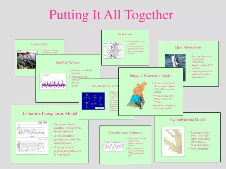
Putting It All Together. Three Assumptions. Vertically integrated primary production is constant across any cross section. Volumetric rates of planktonic community respiration are constant across any cross section.

E N D
Three Assumptions • Vertically integrated primary production is constant across any cross section. • Volumetric rates of planktonic community respiration are constant across any cross section. • Benthic respiration rates in littoral areas are half those in adjacent deep sediments.
MB NB SB
As a sensitivity run, route all mortality and predation to water column as DOC Normally, all mortality and predation goes to sediments as POC
Previous Result Sensitivity Run
KDOC = 0.011/d KDOC = 0.017/d
Run 48 is sensitivity to benthic algal DOC. The rest are sensitivity to KDOC Model High Model Low
Conclusions • Improvement of dissolved oxygen computations in the deep trench requires production of more dissolved organic carbon. • Dissolved oxygen computations are largely insensitive to first-order DOC respiration rate • Investigate DOC production through benthic algae, SAV, deposit feeders, filter feeders
Advanced Optical Model • The model is finished, field work, report completed. • Implemented in water quality model • Parameter set has been updated since initial implementation
Partial Attenuation Model Revised Parameter Set
Partial Attenuation Model Revised Parameter Set
Conclusions • The optical model is implemented and running well • Shortcomings are perhaps more related to the solids calculation than to the optical model • Still, additional parameter refinements are likely
Vallisneria Ruppia Zostera
Zostera Stand-Alone Calibration Leaf Root
Vallisneria Stand-Alone Calibration Ruppia Stand-Alone Calibration
Compensation Irradiance Pm(T) = maximum production at temperature T (g C g-1 DW d-1) Fam = Fraction of production devoted to active metabolism (0 < Fam < 1) Acdw = plant carbon-to-dry-weight ratio (g C g-1 DW) Ic = compensation irradiance (E m-2 d-1) BM = basal metabolism (d-1)
Zostera and Ruppia Marsh et al. (1986). Ic is a function of Temperature
Vallisneria Chesapeake Bay
Zostera Chesapeake Bay
Ruppia Choptank River
Vallisneria Potomac River
Conclusions • The SAV model is reasonably well-calibrated in terms of SAV response to light attenuation • Some tuning is always possible • Final calibration depends on calculation of light attenuation
Bankloads • The bankloads are in. About 11,600 tonnes/day. • Half coarse, half fine. Less than 2% organic system-wide. • Previous loads employed in model were 12,800 kg/day. • Not that different. Why?
Bankloads • Previous shoreline was based on model cell length. 3290 km. • New shoreline is based on map. 7000 km. • Previous load was 3.9 kg/m/d. Now 1.7 kg/m/d. • For now, they are input as daily-average loads.
No Bank Loads With Bank Loads
No Bank Loads With Bank Loads
Suspension-Feeding Benthos • In terms of abundance and distribution, the dominant species are rangia, mya, and corbicula • We received from the Bay Program a data base of more than 10,000 benthos records, 1985 – 2005 • Roughly 1,800 rangia, 800 mya, 250 corbicula, 1985 - 2005
How Do We Place Them? • Consider only CBPS with median AFDW > 10 g/sq m • We know from the oyster model that 2 g AFDW/sq m has no effect on anything • Effect of density < 10 g AFDW/sq m is absorbed into generalized predation term
Where do We Place Them? • Rangia > 10 are found in 22 of 98 CBPS • Mya > 10 are found in 11 of 98 CBPS • Corbicula > 10 are found in 6 of 98 CBPS
What Cells? As per your request for habitat characterization for corbicula,mya and rangia, Based on the book Chesapeake Bay: Nature of the Estuary : A Field Guide by Christopher P. White, Organism Salinity Range Bottom Type Rangia 0.5-10 psu Mud and Sand, like high turbidity areas Mya 5-30 PSU Prefers Sand, but will tolerate Mud Corbicula 0-10 PSU Prefers Sand, but will tolerate clay Sand habitat is defined as an area having < 40 percent silt-clay content.
What Cells? • Bay Program (Kate Hopkins) provided a table of cell versus sand content • Effect of salinity on filtration rate is coded in the model
Is the problem the living resource criterion or the assignment of sand to model cells?