Download
1 / 60
600 likes | 621 Views
Learn about Fourier series, Fourier transform, and discrete Fourier transform in digital image processing. Explore concepts such as convolution property, sampling, Nyquist theorem, and signal reconstruction.

E N D
Digital Image Processing Filtering in the Frequency Domain(Fundamentals) ChristophorosNikou cnikou@cs.uoi.gr
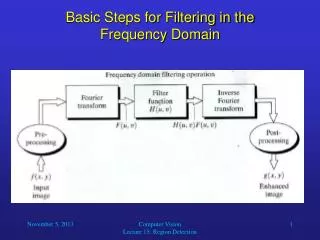
Filtering in the Frequency Domain Filter: A device or material for suppressing or minimizing waves or oscillations of certain frequencies. Frequency: The number of times that a periodic function repeats the same sequence of values during a unit variation of the independent variable. Webster’s New Collegiate Dictionary
Jean Baptiste Joseph Fourier Fourier was born in Auxerre, France in 1768. • Most famous for his work “La Théorie Analitique de la Chaleur” published in 1822. • Translated into English in 1878: “The Analytic Theory of Heat”. Nobody paid much attention when the work was first published. One of the most important mathematical theories in modern engineering.
The Big Idea Images taken from Gonzalez & Woods, Digital Image Processing (2002) = Any function that periodically repeats itself can be expressed as a sum of sines and cosines of different frequencies each multiplied by a different coefficient – a Fourier series
1D continuous signals Images taken from Gonzalez & Woods, Digital Image Processing (2002) • It may be considered both as continuous and discrete. • Useful for the representation of discrete signals through sampling of continuous signals.
1D continuous signals (cont.) Images taken from Gonzalez & Woods, Digital Image Processing (2002) Impulse train function
1D continuous signals (cont.) Images taken from Gonzalez & Woods, Digital Image Processing (2002)
1D continuous signals (cont.) Images taken from Gonzalez & Woods, Digital Image Processing (2002) • The Fourier series expansion of a periodic signal f (t).
1D continuous signals (cont.) Images taken from Gonzalez & Woods, Digital Image Processing (2002) • The Fourier transform of a continuous signal f (t). • Attention: the variable is the frequency (Hz) and not the radial frequency (Ω=2πμ) as in the Signals and Systems course.
1D continuous signals (cont.) Images taken from Gonzalez & Woods, Digital Image Processing (2002)
1D continuous signals (cont.) Images taken from Gonzalez & Woods, Digital Image Processing (2002) • Convolution property of the FT.
1D continuous signals (cont.) Images taken from Gonzalez & Woods, Digital Image Processing (2002) • Intermediate result • The Fourier transform of the impulse train. • It is also an impulse train in the frequency domain. • Impulses are equally spaced every 1/ΔΤ.
1D continuous signals (cont.) Images taken from Gonzalez & Woods, Digital Image Processing (2002) Sampling
1D continuous signals (cont.) Images taken from Gonzalez & Woods, Digital Image Processing (2002) • Sampling • The spectrum of the discrete signal consists of repetitions of the spectrum of the continuous signal every 1/ΔΤ. • The Nyquist criterion should be satisfied.
1D continuous signals (cont.) Images taken from Gonzalez & Woods, Digital Image Processing (2002) Nyquist theorem
1D continuous signals (cont.) Images taken from Gonzalez & Woods, Digital Image Processing (2002) FT of a continuous signal Oversampling Critical sampling with the Nyquist frequency Undersampling Aliasing appears
1D continuous signals (cont.) Images taken from Gonzalez & Woods, Digital Image Processing (2002) • Reconstruction (under correct sampling).
1D continuous signals (cont.) Images taken from Gonzalez & Woods, Digital Image Processing (2002) • Reconstruction • Provided a correct sampling, the continuous signal may be perfectly reconstructed by its samples.
1D continuous signals (cont.) Images taken from Gonzalez & Woods, Digital Image Processing (2002) • Under aliasing, the reconstruction of the continuous signal not correct.
1D continuous signals (cont.) Images taken from Gonzalez & Woods, Digital Image Processing (2002) Aliased signal
The Discrete Fourier Transform Images taken from Gonzalez & Woods, Digital Image Processing (2002) • The Fourier transform of a sampled (discrete) signal is a continuous function of the frequency. • For a N-length discrete signal, taking N samples of its Fourier transform at frequencies: provides the discrete Fourier transform (DFT) of the signal.
The Discrete Fourier Transform (cont.) Images taken from Gonzalez & Woods, Digital Image Processing (2002) • DFT pair of signal f [n] of length N.
The Discrete Fourier Transform (cont.) Images taken from Gonzalez & Woods, Digital Image Processing (2002) • Property • The DFT of a N-length f [n] signal is periodic with period N. • This is due to the periodicity of the complex exponential:
The Discrete Fourier Transform (cont.) Images taken from Gonzalez & Woods, Digital Image Processing (2002) • Property: sum of complex exponentials The proof is left as an exercise.
The Discrete Fourier Transform (cont.) Images taken from Gonzalez & Woods, Digital Image Processing (2002) • DFT pair of signal f [n] of length N may be expressed in matrix-vector form.
The Discrete Fourier Transform (cont.) Example for N=4
The Discrete Fourier Transform (cont.) The inverse DFT is then expressed by: This is derived by the complex exponential sum property.
Linear convolution is of length N=N1+N2-1=4
Circular shift • Signal x[n] of length N. • A circular shift ensures that the resulting signal will keep its length N. • It is a shift modulo N denoted by • Example: x[n] is of length N=8.
Circular convolution g[n]=f [n]h[n] Circular shift modulo N The result is of length
Circular convolution (cont.) g[n]=f [n]h[n]
DFT and convolution g[n]=f [n]h[n] • The property holds for the circular convolution. • In signal processing we are interested in linear convolution. • Is there a similar property for the linear convolution?
DFT and convolution (cont.) g[n]=f [n]h[n] • Letf [n] be of length N1andh[n] be of length N2. • Then g[n]=f [n]*h[n] is of length N1+N2-1. • If the signals are zero-padded to length N=N1+N2-1 then their circular convolution will be the same as their linear convolution: Zero-padded signals
DFT and convolution (cont.) Zero-padding to length N=N1+N2-1 =4 The result is the same as the linear convolution.
DFT and convolution (cont.) Verification using DFT
DFT and convolution (cont.) Element-wise multiplication
DFT and convolution (cont.) Inverse DFT of the result The same result as their linear convolution.
2D continuous signals Images taken from Gonzalez & Woods, Digital Image Processing (2002) Separable:
2D continuous signals (cont.) Images taken from Gonzalez & Woods, Digital Image Processing (2002) The 2D impulse train is also separable:
2D continuous signals (cont.) Images taken from Gonzalez & Woods, Digital Image Processing (2002) • The Fourier transform of a continuous 2D signal f (x,y).
2D continuous signals (cont.) Images taken from Gonzalez & Woods, Digital Image Processing (2002) • Example: FT of f (x,y)=δ(x) y f (x,y)=δ(x) x F(μ,ν)=δ(ν) ν μ
2D continuous signals (cont.) Images taken from Gonzalez & Woods, Digital Image Processing (2002) • Example: FT of f (x,y)=δ(x-y) f (x,y)=δ(x-y) y x F(μ,ν)=δ(μ+ν) ν μ
2D continuous signals (cont.) Images taken from Gonzalez & Woods, Digital Image Processing (2002)
2D continuous signals (cont.) Images taken from Gonzalez & Woods, Digital Image Processing (2002) • 2D continuous convolution • We will examine the discrete convolution in more detail. • Convolution property
2D continuous signals (cont.) Images taken from Gonzalez & Woods, Digital Image Processing (2002) • 2D sampling is accomplished by • The FT of the sampled 2D signal consists of repetitions of the spectrum of the 1D continuous signal.
2D continuous signals (cont.) Images taken from Gonzalez & Woods, Digital Image Processing (2002) • The Nyquist theorem involves both the horizontal and vertical frequencies. Under-sampled Over-sampled
Aliasing Images taken from Gonzalez & Woods, Digital Image Processing (2002)
Aliasing - Moiré Patterns • Effect of sampling a scene with periodic or nearly periodic components (e.g. overlapping grids, TV raster lines and stripped materials). • In image processing the problem arises when scanning media prints (e.g. magazines, newspapers). • The problem is more general than sampling artifacts.