Download

1 / 65
661 likes | 807 Views
Frequency Filtering. Instructor: Juyong Zhang juyong@ustc.edu.cn http://staff.ustc.edu.cn/~juyong. Convolution Property of the Fourier Transform. * = convolution · = multiplication.

E N D
Frequency Filtering Instructor: Juyong Zhang juyong@ustc.edu.cn http://staff.ustc.edu.cn/~juyong
Convolution Property of the Fourier Transform * = convolution · = multiplication The Fourier Transform of a convolution equals the product of the Fourier Transforms. Similarly, the Fourier Transform of a convolution is the product of the Fourier Transforms
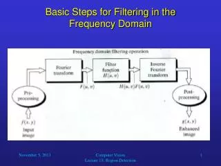
Convolution via Fourier Transform Image & Mask Transforms Pixel-wise Product Inverse Transform
How to Convolve via FT in Matlab • Read the image from a file into a variable, say I. • Read in or create the convolution mask, h. • Compute the sum of the mask: s = sum(h(:)); • If s == 0, set s = 1; • Replace h with h = h/s; • Create: H = zeros(size(I)); • Copy h into the middle of H. • Shift Hinto position: H = ifftshift(H); • Take the 2D FT of I and H:FI=fft2(I); FH=fft2(H); • Pointwise multiply the FTs: FJ=FI.*FH; • Compute the inverse FT: J = real(ifft2(FJ)); The mask is usually 1-band For color images you may need to do each step for each band separately.
Even Odd Even Odd Image Origin Image Origin Weight Matrix Origin Weight Matrix Origin After FFT shift After FFT shift After IFFT shift After IFFT shift Coordinate Origin of the FFT Center = (floor(R/2)+1, floor(C/2)+1)
J = fftshift(I): I(1,1) J ( R/2 +1, C/2 +1) I = ifftshift(J): J( R/2 +1, C/2 +1) I(1,1) Matlab’s fftshift and ifftshift where x = floor(x) = the largest integer smaller than x.
Blurring: Averaging / Lowpass Filtering Blurring results from: • Pixel averaging in the spatial domain: • Each pixel in the output is a weighted average of its neighbors. • Is a convolution whose weight matrix sums to 1. • Lowpass filtering in the frequency domain: • High frequencies are diminished or eliminated • Individual frequency components are multiplied by a nonincreasing function of such as 1/ = 1/(u2+v2). The values of the output image are all non-negative.
Sharpening: Differencing / Highpass Filtering Sharpening results from adding to the image, a copy of itself that has been: • Pixel-differenced in the spatial domain: • Each pixel in the output is a difference between itself and a weighted average of its neighbors. • Is a convolution whose weight matrix sums to 0. • Highpass filtered in the frequency domain: • High frequencies are enhanced or amplified. • Individual frequency components are multiplied by an increasing function of such as = (u2+v2), where is a constant. The values of the output image positive & negative.
Recall: Convolution Property of the Fourier Transform * = convolution · = multiplication The Fourier Transform of a convolution equals the product of the Fourier Transforms. Similarly, the Fourier Transform of a convolution is the product of the Fourier Transforms
Ideal Lowpass Filter Image size: 512x512 FD filter radius: 16 Multiply by this, or … … convolve by this Fourier Domain Rep. Spatial Representation Central Profile
Ideal Lowpass Filter Image size: 512x512 FD filter radius: 8 Multiply by this, or … … convolve by this Fourier Domain Rep. Spatial Representation Central Profile
Consider the image below: Power Spectrum and Phase of an Image Original Image Power Spectrum Phase
Ideal Lowpass Filter Image size: 512x512 FD filter radius: 16 Ideal LPF in FD Original Image Power Spectrum
Ideal Lowpass Filter Image size: 512x512 FD filter radius: 16 Original Image Filtered Power Spectrum Filtered Image
Ideal Highpass Filter Image size: 512x512 FD notch radius: 16 Multiply by this, or … … convolve by this Fourier Domain Rep. Spatial Representation Central Profile
Ideal Highpass Filter Image size: 512x512 FD notch radius: 16 Power Spectrum Original Image Ideal HPF in FD
*signed image: 0 mapped to 128 Ideal Highpass Filter Image size: 512x512 FD notch radius: 16 Original Image Filtered Power Spectrum Filtered Image*
*signed image: 0 mapped to 128 Ideal Highpass Filter Image size: 512x512 FD notch radius: 16 Positive Pixels Filtered Image* Negative Pixels
Ideal Bandpass Filter • A bandpass filter is created by • subtracting a FD radius 2 lowpass filtered image from a FD radius 1 lowpass filtered image, where 2< 1, or • convolving the image with a mask that is the difference of the two lowpass masks. - = FD LP mask with radius 1 FD LP mask with radius 2 FD BP mask 1 -2
*signed image: 0 mapped to 128 Ideal Bandpass Filter image LPF radius 1 image LPF radius 2 image BPF radii 1, 2*
*signed image: 0 mapped to 128 Ideal Bandpass Filter original image* filter power spectrum filtered image
*signed image: 0 mapped to 128 A Different Ideal Bandpass Filter original image filter power spectrum filtered image*
The Uncertainty Relation space frequency FT space frequency FT A small object in space has a large frequency extent and vice-versa.
The Uncertainty Relation frequency space Recall: a symmetric pair of impulses in the frequency domain becomes a sinusoid in the spatial domain. IFT small extent large extent small extent large extent frequency space A symmetric pair of lines in the frequency domain becomes a sinusoidal line in the spatial domain. IFT small extent large extent small extent large extent
Ideal Filters Do Not Produce Ideal Results IFT A sharp cutoff in the frequency domain… …causes ringing in the spatial domain.
Ideal Filters Do Not Produce Ideal Results Ideal LPF Blurring the image above with an ideal lowpass filter… …distorts the results with ringing or ghosting.
Optimal Filter: The Gaussian IFT The Gaussian filter optimizes the uncertainty relation. It provides the sharpest cutoff with the least ringing.
R = 512, C = 512 c r = 257, s= 64 Two-Dimensional Gaussian If and are different for r & c… …or if and are the same for r & c.
Optimal Filter: The Gaussian Gaussian LPF With a gaussian lowpass filter, the image above … … is blurred without ringing or ghosting.
Compare with an “Ideal” LPF Ideal LPF Blurring the image above with an ideal lowpass filter… …distorts the results with ringing or ghosting.
Gaussian Lowpass Filter Image size: 512x512 SD filter sigma = 8 Multiply by this, or … … convolve by this Fourier Domain Rep. Spatial Representation Central Profile
Gaussian Lowpass Filter Image size: 512x512 SD filter sigma = 2 Multiply by this, or … … convolve by this Fourier Domain Rep. Spatial Representation Central Profile
Gaussian Lowpass Filter Image size: 512x512 SD filter sigma = 8 Power Spectrum Original Image Gaussian LPF in FD
Gaussian Lowpass Filter Image size: 512x512 SD filter sigma = 8 Original Image Filtered Power Spectrum Filtered Image
Gaussian Highpass Filter Image size: 512x512 FD notch sigma = 8 Multiply by this, or … … convolve by this Fourier Domain Rep. Spatial Representation Central Profile
Gaussian Highpass Filter Image size: 512x512 FD notch sigma = 8 Power Spectrum Original Image Gaussian HPF in FD
*signed image: 0 mapped to 128 Gaussian Highpass Filter Image size: 512x512 FD notch sigma = 8 Original Image Filtered Power Spectrum Filtered Image*
*signed image: 0 mapped to 128 Gaussian Highpass Filter Image size: 512x512 FD notch sigma = 8 Negative Pixels Positive Pixels Filtered Image*
*signed image: 0 mapped to 128 Another Gaussian Highpass Filter original image filter power spectrum filtered image*
Gaussian Bandpass Filter • A bandpass filter is created by • subtracting a FD radius 2 lowpass filtered image from a FD radius 1 lowpass filtered image, where 2< 1, or • convolving the image with a mask that is the difference of the two lowpass masks. - = FD LP mask with radius 1 FD LP mask with radius 2 FD BP mask 1 -2
*signed image: 0 mapped to 128 Ideal Bandpass Filter original image filter power spectrum filtered image*
*signed image: 0 mapped to 128 Gaussian Bandpass Filter image LPF radius 1 image LPF radius 2 image BPF radii 1, 2*