Download
1 / 21
220 likes | 441 Views
Basic Steps for Filtering in the Frequency Domain. Noisy image. Noise-cleaned image. Fourier spectrum. Noise Removal. Low Pass Filtering. Original. Low Pass Butterworth 50% cutoff diameter 10 (left) and 25. High Pass Filtering. Original. High Pass Butterworth

E N D
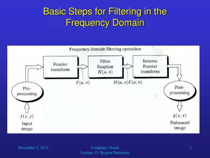
Basic Steps for Filtering in the Frequency Domain Computer Vision Lecture 15: Region Detection
Noisy image Noise-cleaned image Fourier spectrum Noise Removal Computer Vision Lecture 15: Region Detection
Low Pass Filtering Original Low Pass Butterworth 50% cutoff diameter 10 (left) and 25 Computer Vision Lecture 15: Region Detection
High Pass Filtering Original High Pass Butterworth 50% cutoff diameter 10 (left) and 25 Computer Vision Lecture 15: Region Detection
Motion Blurring Filter Aerial photo blurred by motion and its spectrum The blur vector and its spectrum Computer Vision Lecture 15: Region Detection
Motion Blurring Filter The result of dividing the original spectrum by the motion spectrum and then retransforming Computer Vision Lecture 15: Region Detection
Convolution Theorem • Let F {.} denote the application of the Fourier transform and * denote convolution (as usual). • Then we have: • F {(f*h)(x, y)} = F(u, v) H(u, v) and • F {f(x,y) h(x, y)} = (F*H)(u, v), • where F and H are the Fourier transformed images f and h, respectively. • This means that instead of computing the convolution directly, we can Fourier transform f and h, multiply them, and then transform them back. • In other words, a convolution in the space domain corresponds to a multiplication in the frequency domain, and vice versa. Computer Vision Lecture 15: Region Detection
Demo Website • I highly recommend taking a look at this website: • http://users.ecs.soton.ac.uk/msn/book/new_demo/ • It has nice interactive demonstrations of the Fourier transform, the Hough transform, edge detection, and many other useful operations. Computer Vision Lecture 15: Region Detection
Region Detection • There are two basic – and often complementary – approaches to segmenting an image into individual objects or parts of objects: region-based segmentation and boundary estimation. • Region-based segmentation is based on region detection, which we will discuss in this lecture. • Boundary estimation is based on edge detection, which we already discussed earlier. Computer Vision Lecture 15: Region Detection
Region Detection • We have already seen the simplest kind of region detection. • It is the labeling of connected components in binary images. • Of course, in general, region detection is not that simple. • Successful region detection through component labeling requires that we can determine an intensity threshold in such a way that all objects consist of 1-pixels and do not touch each other. Computer Vision Lecture 15: Region Detection
Region Detection • We will develop methods that can do a better job at finding regions in real-world images. • In our discussion we will first address the question of how to segment an image into regions. • Afterwards, we will look at different ways to represent the regions that we detected. Computer Vision Lecture 15: Region Detection
Region Detection • How shall we define regions? • The basic idea is that within the same region the intensity, texture, or other features do not change abruptly. • Between adjacent regions we do find such a change in at least one feature. • Let us now formalize the idea of partitioning an image into a set of regions. Computer Vision Lecture 15: Region Detection
Region Detection • A partition S divides an image I into a set of n regions Ri. Regions are sets of connected pixels meeting three requirements: • The union of regions includes all pixels in the image, • Each region Ri is homogeneous, i.e., satisfies a homogeneity predicate P so that P(Ri) = True. • The union of two adjacent regions Ri and Rj never satisfies the homogeneity predicate, i.e., P(Ri Rj) = False. Computer Vision Lecture 15: Region Detection
Region Detection The homogeneity predicate could be defined as, for example, the maximum difference in intensity values between two pixels being no greater than a some threshold . Usually, however, the predicate will be more complex and include other features such as texture. Also, the parameters of the predicate such as may be adapted to the properties of the image. Let us take a look at the split-and-merge algorithm of image segmentation. Computer Vision Lecture 15: Region Detection
The Split-and-Merge Algorithm • First, we perform splitting: • At the start of the algorithm, the entire image is considered as the candidate region. • If the candidate region does not meet the homogeneity criterion, we split it into four smaller candidate regions. • This is repeated until there are no candidate regions to be split anymore. • Then, we perform merging: • Check all pairs of neighboring regions and merge them if it does not violate the homogeneity criterion. Computer Vision Lecture 15: Region Detection
The Split-and-Merge Algorithm • Sample image to be segmented with = 1 Computer Vision Lecture 15: Region Detection
The Split-and-Merge Algorithm • First split Computer Vision Lecture 15: Region Detection
The Split-and-Merge Algorithm • Second split Computer Vision Lecture 15: Region Detection
The Split-and-Merge Algorithm • Third split Computer Vision Lecture 15: Region Detection
The Split-and-Merge Algorithm • Merge Computer Vision Lecture 15: Region Detection
The Split-and-Merge Algorithm • Final result Computer Vision Lecture 15: Region Detection