Download
1 / 9

E N D
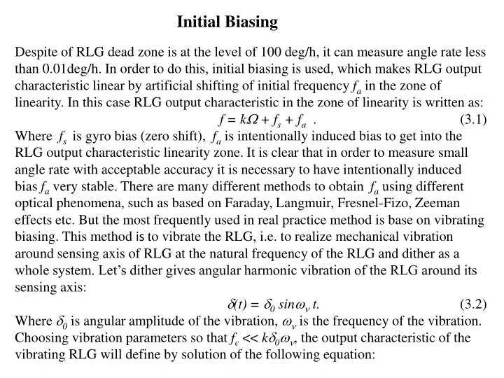
Initial Biasing Despite of RLG dead zone is at the level of 100 deg/h, it can measure angle rate less than 0.01deg/h. In order to do this, initial biasing is used, which makes RLG output characteristic linear by artificial shifting of initial frequencyfa in the zone of linearity. In this case RLG output characteristic in the zone of linearity is written as: f = k + fs + fa. (3.1) • Where fsis gyro bias (zero shift), fa is intentionally induced bias to get into the RLG output characteristic linearity zone.It is clear that in order to measure small angle rate with acceptable accuracy it is necessary to have intentionally induced biasfa very stable. There are many different methods to obtain fa using different optical phenomena, such as based on Faraday,Langmuir, Fresnel-Fizo, Zeeman effects etc. But the most frequently used in real practice method is base on vibrating biasing. This method is to vibrate the RLG, i.e. to realize mechanical vibration around sensing axis of RLG at the natural frequency of the RLG and dither as a whole system. Let’s dither gives angular harmonic vibration of the RLG around its sensing axis: • (t) = 0 sin t. (3.2) • Where 0 is angular amplitude of the vibration, is the frequency of the vibration. Choosing vibration parameters so that fc << k0, the output characteristic of the vibrating RLG will define by solution of the following equation:
f cd d0 • Fig. 3.1. RLG dynamic lock-in threshold. (3.3) • Here phase difference averaged over vibration period, J0- Bessel function of the zero order. So, for vibrating biasing frequency difference of the counter propagated waves is defined from the relationship: • fcd = fc |Jo (k0 )|. (3.4) value fcd is called dynamic lock-in threshold. The dependence of dynamic lock-in threshold on vibration amplitude is presented in fig. 3.1. As can be seen from this figure at certain amplitudes lock-in threshold is equal to zero. However, due to high steepness of the curve Jo(0) in theclose to zero point, zero lock-in threshold cannot be realized in practice because random oscillation of vibration amplitude results in that fcd 0. For large 0 when k0>>1 dynamic lock-in threshold is approximately defined from the relationship: (3.5) For example, for k = 0.5 pulse/arc.sec, 0= 10 arc.min andfc = 1000 Hz dynamic lock-in threshold isfcd= 50 Hz, i.e. 20 times less than static threshold.
f w 4 v w 3 v w 2 v w v W W 2 cd W 2 c Fig. 3.2. Vibrating RLG output characteristic. At the same time with diminishing of lock-in threshold of vibrating RLG on its output characteristic appear the “shelves”, due to synchronization of difference frequency with RLG vibration harmonics as depicted in fig.3.2. The presence of the “shelves” leads to additional requirement, apart from 0 >>1 it is necessary that 0 >> 1. When RLG mechanical vibration spectrum is wide and the “shelves” become smaller and appear more often, then quasi-harmonic linearization of vibrating RLG output characteristic is realized. As practice showed, small addition of random component in periodic vibration is sufficient to get acceptable for application linearity of output characteristic. Vibration biasing requires that angle rate read-out time would be in accordance with vibration period, so that reversible counting of pulses for read-out time is equal to multiple of vibration period. In this case angle rate of induced vibration is driven to null and only angle rate measured remains.
Rate Biasing • There is one more very simple biasing that is used in practice to design gyrocompass with autocompensation property. It is so-called rate biasing, with the rate value sufficient to get to linearity region of the RLG output characteristic. In this case fa= k0cos, where 0 is induced rotation rate, is the angle between the induced rotation rate vector and RLG sensing axis. To reach high stability of fa in this case read-out time is given by angle encoder and stability of fa is dependent on accuracy of angle encoder. There are many high accuracy optical encoders which can provide very stable frequency (rate) biasing fa.
Gyro Accuracy Parameters By analogy with electromechanical gyros, accuracy characteristic of any gyro is expressed in unities of angle rate. The main accuracy characteristic of any gyro including RLG is bias stability or bias drift. Electromechanical gyro drift is characterized by angular motion of the kinetic momentum vector in inertial space and can be directly measured. Modern gyros measurement errors can be measured only by output signal and then reduced to its input. In order to reduce gyro errors to the input it is necessary to know its scale factor. Usage of scale factor introduces additional errors in accuracy characteristics of gyros. However, taking into account lower influence of scale factor error when calculating bias error (SFbias<<1), bias drift can be reduce to gyro input (that is expressed in deg/h or deg/s) with negligible error. Fig.3.3 shows typical behavior of the bias during warming process right after power is on. • Bias instability from sample to sample and from turn-on to turn-on defines bias repeatability. So, turn-on to turn-on bias instability is very important accuracy characteristic of any gyro and this value is written down in gyro technical passport. In run bias stability is also important accuracy characteristic which is written down in the device’s passport. In modern RLG these accuracy parameters are in the range of [1…0.01] deg/h.
Bias repeatability N(t) 5.4s0 s0=(fmax-fmin)/5.4K t tw Warmed-up time Fig.3.3. Typical gyro drift during warming-up. N(t) Root mean square value of bias drift • t=it sdr=(fmax-fmin)/5.4K 5.4sdr t Fig.3.4. Typical gyro drift after warmed-up. In-run bias instability has many components, but the most important are two of them: short term bias instability and random walk. Short term bias stability (or instability) can be defined by two ways. The first way is that gyro output signal at zero input angle rate is divided by 100 s interval clusters and calculate average value for each cluster, then calculate root mean square (RMS) value, , for obtained averaged measurements. Fig.3.4 shows typical in-run bias stability for any gyro. 100 s Mi
Random walk=0.017 deg/h1/2 Allan variance curve tan=-0.5 Drift by Allan=min()=0.17 deg/h , Fig.3.5. Allan variance of gyro output signal The second way uses Allan variance method recommended by international IEEE standard (for example, IEEE Std 952-1997(R2003) and Std.1431TM-2004). The essence of this method is that the n measurements are divided by p clusters m measurements in each. (3.6) Where Niis i-thmeasurement with sample time t, =mt – averaging time.Usually L=5-10. Then RMS value, (p), of Mp should be calculated as follows: (3.7) 2 is called Allan variance. Then the graph of on should be drawn in log-log axes. Typical graph of on of any gyro resembles parabola as can be seen in fig 3.5. Minimum in this graph determines gyro drift, and straight line tangential to Allan variance curve with tilt angle such as tan()=-0.5 determines gyro random walk value.
Another noise-like short term bias instability characteristic is random walk. It is equivalent to Brownian noise in physics. This noise results from quantization noise, electronic thermal noise and technical fluctuation of the difference frequency. For modern RLG root mean square deviation () is in the range [0.5… 0.002]deg/h. It means that integrating RLG output signal over 1 hour the error of angle measurement is equal to 0.002 deg only for the account of random component (noise). It is supposed that random error is accumulated during integration of output signal as rwt1/2. The gyro drift often call as systematic error because it changes with ultra low frequency, less than 0.01 Hz. It is like flicker noise in electronics. All components of bias instability present additive errors. Additive gyro errors can be described by the following model: x(t) = b + at + (t). (3.8) Here b is the gyro bias having nonzero value and standard deviation, b, from turn-on to turn-on which characterizes bias repeatability; a is the bias drift rate (trend) which characterizes in-run bias instability and changes from turn-on to turn-on having standard deviation a; (t) is random component which characterizes noise i.e. random walk.
Table 3.1 shows world leading RLG manufacturers and RLG main parameters. Table 3.1