Download
1 / 67
670 likes | 795 Views
Organizing and describing Data. Instructor:. W.H.Laverty. Office:. 235 McLean Hall. Phone:. 966-6096. Lectures:. M W F 11:30am - 12:20pm Arts 143 Lab: M 3:30 - 4:20 Thorv105. Evaluation:. Assignments, Labs, Term tests - 40% Every 2nd Week (approx) – Term Test Final Examination - 60%.

E N D
Instructor: W.H.Laverty Office: 235 McLean Hall Phone: 966-6096 Lectures: M W F 11:30am - 12:20pm Arts 143 Lab: M 3:30 - 4:20 Thorv105 Evaluation: Assignments, Labs, Term tests - 40% Every 2nd Week (approx) – Term TestFinal Examination - 60%
Techniques for continuous variables Continuous variables are measurements that vary over a continuum (Weight, Blood Pressure, etc.) (as opposed to categorical variables Gender, religion, Marital Status etc.)
To Construct • A Grouped frequency table • A Histogram
Find the maximum and minimum of the observations. • Choose non-overlapping intervals of equal width (The Class Intervals) that cover the range between the maximum and the minimum. • The endpoints of the intervals are called the class boundaries. • Count the number of observations in each interval (The cell frequency - f). • Calculate relative frequency relative frequency = f/N
Data Set #3 The following table gives data on Verbal IQ, Math IQ, Initial Reading Acheivement Score, and Final Reading Acheivement Score for 23 students who have recently completed a reading improvement program Initial Final Verbal Math Reading Reading Student IQ IQ Acheivement Acheivement 1 86 94 1.1 1.7 2 104 103 1.5 1.7 3 86 92 1.5 1.9 4 105 100 2.0 2.0 5 118 115 1.9 3.5 6 96 102 1.4 2.4 7 90 87 1.5 1.8 8 95 100 1.4 2.0 9 105 96 1.7 1.7 10 84 80 1.6 1.7 11 94 87 1.6 1.7 12 119 116 1.7 3.1 13 82 91 1.2 1.8 14 80 93 1.0 1.7 15 109 124 1.8 2.5 16 111 119 1.4 3.0 17 89 94 1.6 1.8 18 99 117 1.6 2.6 19 94 93 1.4 1.4 20 99 110 1.4 2.0 21 95 97 1.5 1.3 22 102 104 1.7 3.1 23 102 93 1.6 1.9
In this example the upper endpoint is included in the interval. The lower endpoint is not.
Example • In this example we are comparing (for two drugs A and B) the time to metabolize the drug. • 120 cases were given drug A. • 120 cases were given drug B. • Data on time to metabolize each drug is given on the next two slides
To Construct • A Grouped frequency table • A Histogram
To Construct - A Grouped frequency table • Find the maximum and minimum of the observations. • Choose non-overlapping intervals of equal width (The Class Intervals) that cover the range between the maximum and the minimum. • The endpoints of the intervals are called the class boundaries. • Count the number of observations in each interval (The cell frequency - f). • Calculate relative frequency relative frequency = f/N
To draw - A Histogram Draw above each class interval: • A vertical bar above each Class Interval whose height is either proportional to The cell frequency (f) or the relative frequency (f/N) frequency (f) or relative frequency (f/N) Class Interval
Some comments about histograms • The width of the class intervals should be chosen so that the number of intervals with a frequency less than 5 is small. • This means that the width of the class intervals can decrease as the sample size increases
If the width of the class intervals is too small. The frequency in each interval will be either 0 or 1 • The histogram will look like this
If the width of the class intervals is too large. One class interval will contain all of the observations. • The histogram will look like this
Ideally one wants the histogram to appear as seen below. • This will be achieved by making the width of the class intervals as small as possible and only allowing a few intervals to have a frequency less than 5.
As the sample size increases the histogram will approach a smooth curve. • This is the histogram of the population
Comment: the proportion of area under a histogram between two points estimates the proportion of cases in the sample (and the population) between those two values.
Example: The following histogram displays the birth weight (in Kg’s) of n = 100 births
Find the proportion of births that have a birthweight less than 0.34 kg.
The Characteristics of a Histogram • Central Location (average) • Spread (Variability, Dispersion) • Shape
The Stem-Leaf Plot An alternative to the histogram
Each number in a data set can be broken into two parts • A stem • A Leaf
Example Verbal IQ = 84 84 • Stem = 10 digit = 8 • Leaf = Unit digit = 4 Leaf Stem
Example Verbal IQ = 104 104 • Stem = 10 digit = 10 • Leaf = Unit digit = 4 Leaf Stem
To Construct a Stem- Leaf diagram • Make a vertical list of “all” stems • Then behind each stem make a horizontal list of each leaf
Example The data on N = 23 students Variables • Verbal IQ • Math IQ • Initial Reading Achievement Score • Final Reading Achievement Score
Data Set #3 The following table gives data on Verbal IQ, Math IQ, Initial Reading Acheivement Score, and Final Reading Acheivement Score for 23 students who have recently completed a reading improvement program Initial Final Verbal Math Reading Reading Student IQ IQ Acheivement Acheivement 1 86 94 1.1 1.7 2 104 103 1.5 1.7 3 86 92 1.5 1.9 4 105 100 2.0 2.0 5 118 115 1.9 3.5 6 96 102 1.4 2.4 7 90 87 1.5 1.8 8 95 100 1.4 2.0 9 105 96 1.7 1.7 10 84 80 1.6 1.7 11 94 87 1.6 1.7 12 119 116 1.7 3.1 13 82 91 1.2 1.8 14 80 93 1.0 1.7 15 109 124 1.8 2.5 16 111 119 1.4 3.0 17 89 94 1.6 1.8 18 99 117 1.6 2.6 19 94 93 1.4 1.4 20 99 110 1.4 2.0 21 95 97 1.5 1.3 22 102 104 1.7 3.1 23 102 93 1.6 1.9