Download
1 / 21
210 likes | 270 Views
Organizing Data. Essentials Measures of Position Five-Number-Summary Example Box and Whiskers Plots Example Pearson’s Index of Skewness Example Z-scores Example Coefficient of Variation Example. Measures of Position & Exploratory Data Analysis.

E N D
Organizing Data • Essentials • Measures of Position • Five-Number-Summary • Example • Box and Whiskers Plots • Example • Pearson’s Index of Skewness • Example • Z-scores • Example • Coefficient of Variation • Example Measures of Position & Exploratory Data Analysis
Essentials:Measures of Position(Better understanding distribution shapes.) • Know the types of measures used to look at specific positions within a data distribution. • Be able to calculate the inter-quartile range, three quartiles, Pearson’s Index of Skewness, z-score, Coefficient of Variation. • Be familiar with symmetry vs. skewness and distribution shapes. • Be able to build both traditional and modified box plots (aka: box-and-whiskers plot).
Measures of Position • Measures of position are points within the data that are used to describe characteristics of the data. Percentiles, Deciles, Quartiles, Minimum and Maximum are among these points. • We will focus on 5 specific values...
The Five-Number-Summary • Five numbers are frequently used to indicate positions within a data set and much more... • These points are: • Minimum - Q1 - Median - Q3 - Maximum
The Minimum and Maximum values represent the extremes in the data set. Obtaining these points is a simple matter of looking for them. Q1, Median (Q2), and Q3 represent points within the data. They are the 25th, 50th, and 75th percentiles, respectively. Formulas are used to locate these positions. Components of theFive-Number Summary
The Quartiles • The Quartiles are obtained using the following three formulas. • Q1(25th percentile) = (n+1)/4 • Median (Q2, 50th percentile) = (n+1)/2 • Q3 (75th percentile) = [3(n+1)]/4 • (Where n = number of observations. Note that these formulas identify POSITIONS within the data, not values; the data must be placed in numeric order)
The Interquartile Range • The Interquartile Range (IQR) describes the middle 50% of the data. It is obtained by the formula: • IQR = Q3 - Q1 • The Interquartile Range is used as a measure of variation around the Median of a set of data.
Quartiles divide a data set that has been ordered from smallest to largest into four sections, each containing 25% of the data values. A term more familiar to you might be percentile. For example, the 25th percentile, 50th percentile, or 75th percentile. Recall that the median in this data set is found using the formula (n+1)/2 to obtain the POSITION of the median (here the POSITION is (20 + 1)/2 = 10.5). Determining the value half way between the 10th and 11th values yields a Median of 558: [(554 + 562)/2 = 558]. Another name for the median, is the second quartile (Q2) . It is the value in the data set such that 50% of the values are lower than it, and 50% of the values are higher than it. The third quartile (Q3) is the value such that 75% of the values are lower than it, and 25% of the values are higher than it. To find this value apply the formula [3(n+1)/4] to obtain the POSITION of the third quartile. Here the formula yields POSITION 15.75: [(3(20+1))/4 = 15.75]. Determine the value ¾ of the way between the 15th value (638) and the 16th value (664) by determining the difference between these two numbers (664 - 638 = 26); multiplying the difference by .75 (26 * .75 = 19.5); and adding this value to the smaller number (638 + 19.5 = 657.5 = Q3) The first quartile (Q1) is the value such that 25% of the values are lower than it, and 75% of the values are higher than it. To find this value apply the formula (n+1)/4 to obtain the POSITION of the first quartile. Here the formula yields POSITION 5.25: [(20+1)/4 = 5.25]. Determine the value ¼ of the way between the 5th value (483) and the 6th value (514) by determining the difference between these two numbers (514 – 483 = 31); multiplying the difference by .25 (31 * .25 = 7.75); and adding this value to the smaller number (483 + 7.75 = 490.75 = Q1) The Interquartile Range is the difference between the third quartile, and the first quartile. Here, the interquartile range is 657.5 - 490.75 = 166.75 The Minimum value, First Quartile (Q1), Median (Q2), Third Quartile (Q3) and Maximum value comprise what is referred to as the Five Number Summary. Each component of this summary represents a measure of position within a set of data. Together, these five values are referred to as the Five Number Summary. Anatomy of Measures of Position 440 481 482 483 483 514 514 554 554 554 562 612 623 631 638 664 671 677 690 707
Exploring and Comparing Data • Exploratory Data Analysis (EDA): EDA is the process of using statistical tools (graphs, measures of center, variation, and position) to investigate data sets in order to understand their important characteristics.
Box-and-Whiskers Plot • a.k.a. Box plot • A Box plot is used to display the five-number-summary. One can also examine the shape of the distribution with a Box plot. • Data Presentation: • Box plot: Traditional vs. Modified Box plot • Display of Outliers and Adjacent Values
Anatomy of a Traditional Box plot DUDLEY’S DOUGHNUTS (flour in pounds, used on 20 consecutive days during the month of Dec. 1999) Title This is Q3, the third quartile. Here, Q3 is 657.5. This is the Upper Whisker. It is the maximum value in the data set. Here, the maximum value is 707. This is the Median (Q2).Here, the median is 558. This is the Lower Whisker. It is the minimum value in the data set. Here, the minimum value is 440. This is Q1, the first quartile. Here, Q1 is 490.75. Flour (in lbs.) Used 440, 481, 482, 483, 483, 514, 514, 554, 554, 554, 562, 612, 623, 631, 638, 664, 671, 677, 690, 707 Historical Note Who invented this useful tool for quick data analysis? John Tukey Statistician
Outliers, Limits, and Adjacent Points • An Outlier is a data point found at one of the extremes of the data, and is well outside the general pattern of the data. • Upper and Lower Limits: Used as a tool to identify observations that may be outliers. • Lower Limit = Q1 - 1.5(IQR) • Upper Limit = Q3 + 1.5(IQR) • Adjacent Points: The last data value that occurs before (or at) the Upper or Lower Limit. In modified Box plots the whisker would stop at this data value rather than being drawn out to 1.5(IQR).
Mean Price of a Movie Ticket for a Sample of 12 U.S. Cities Example of a Modified Box Plot
A grouped box plot is a good way to visualize differences/similarities between groups. Grouped Box plots
Pearson’s Index of Skewness • Skewness can be measured using Pearson’s Index of Skewness. • Example: Given a set of date whose statistics include: mean = 40, median = 41, S.D = 4, determine if this distribution id skewed. • I = (3(40 - 41))/4 = -.75 • Given that the value is within the range from -1 to 1, inclusive, this distribution would not be considered to be significantly skewed.
Pearson’s Index of Skewness • When symmetric, I = 0. • Values usually range from –3 to +3. • A distribution is considered symmetric if the index value is between -1 and +1 • If the index value (I) is less than -1 the data are negatively (left) skewed. • If the index value is greater than +1 The data are positively (right) skewed.
Pearson’s Index of Skewness: Example Use Pearson’s Index of Skewness to determine if the distribution of 406 automobile weights is approximately normally distributed or does it display a degree of skewness? Mean Wt: 2969.56 lb. Median Wt: 2811.00 lb. Standard Deviation: 849.83 lb.
Measures of Position • Standard Scores: a standard score, or z-score is the number of standard deviations that a given value x is above or below the mean. To find a z-score For populations: For samples: (Always round z to two decimal places.)
Standard Scores (z-score) Recall, a z-score is a measure of a value’s distance away from a distribution’s mean as measured in standard deviations. • Example: Ozzie just took two tests. Given his scores, the mean for the tests, and the standard deviations, on which test did Ozzie perform better relative to the other students? • Calculus Exam: Grade = 65, class mean = 50, S.D. = 10 • z = (65 - 50)/10 = 1.5 (or 1.5 standard deviations above the mean) • History exam: Grade = 30, class mean = 25, S.D. = 5 • z = (30 - 25)/5 = 1 (or 1 standard deviation above the mean) • Since the z-score for the calculus exam is larger, Ozzie’s relative position is higher in the calculus class than it is in the history class.
Coefficient of Variation • Allows us to compare standard deviations. The result is expressed as a percentage. • Example:Trinity’s test statistics included: Anthropology test - mean of 50 and S.D. of 10; Music test - mean of 40 and S.D. of 5. Which test showed greater variation in test scores? • Anthropology: (10/50)*100 = 20% • Music: (5/40)*100 = 12.5% • Thus, there was greater variation in test scores for the Anthropology test.
Coefficient of Variation: Example • The heights and weights and ages of the starting members of the 2008 World Champion Boston Celtics are noted below. Determine the coefficient of determination for these variables to determine which has the greatest variation. • Ray Allen: 77 in., 205 lb., 33 yrs. • Rajon Rondo: 73 in., 171 lb., 21 yrs. • Paul Pierce: 79 in., 235 lb., 30 yrs. • Kevin Garnett: 83 in., 253 lb., 32 yrs. • Kendrick Perkins: 82 in., 280 lb., 23 yrs.